Shannon's sampling theory, showing that a bandlimited signal f(x) could be ..... down the system's equations is that we have to deal with a multirate system ...
TO APPEAR IN IEEE TRANSACTIONS ON CIRCUITS AND SYSTEM II
1
A Generalized Sampling Theory without bandlimiting constraints Michael Unser and Josiane Zerubia Abstract— We consider the problem of the reconstruction of a continuous-time function f (x) ∈ H from the samples of the responses of m linear shift-invariant systems sampled at 1/m the reconstruction rate. We extend Papoulis’ generalized sampling theory in two important respects. First, our class of admissible input signals (typ. H = L2 ) is considerably larger than the subspace of bandlimited functions. Second, we use a more general specification of the reconstruction subspace V (ϕ), so that the output of the system can take the form of a bandlimited function, a spline, or a wavelet expansion. Since we have enlarged the class of admissible input functions, we have to give up Shannon and Papoulis’ principle of an exact reconstruction. Instead, we seek an approximation f˜ ∈ V (ϕ) that is consistent in the sense that it produces exactly the same measurements as the input of the system. This leads to a generalization of Papoulis’ sampling theorem and a practical reconstruction algorithm that takes the form of a multivariate filter. In particular, we show that the corresponding system acts as a projector from H onto V (ϕ). We then propose two complementary polyphase and modulation domain interpretations of our solution. The polyphase representation leads to a simple understanding of our reconstruction algorithm in terms of a perfect reconstruction filterbank. The modulation analysis, on the other hand, is useful in providing the connection with Papoulis’ earlier results for the bandlimited case. Finally, we illustrate the general applicability of our theory by presenting new examples of interlaced and derivative sampling using splines.
Michael Unser is with the Swiss Federal Institute of Technology, EPFL - DMT/IOA, CH-1015 Lausanne, Switzerland. Josiane Zerubia is with INRIA, 2004 route des Lucioles, F-06902 Sophia Antipolis, France.
GLOSSARY OF SYMBOLS f (x) : unknown input signal; f˜(x) : reconstructed signal approximation; H : input space; V (ϕ) : reconstruction subspace; ϕ(x) : generating function; aϕ (k) = hϕ(x − k), ϕ(x)i : autocorrelation sequence; b aϕ (ejω ) : Fourier transform of aϕ (k); Aϕ , Bϕ : Riesz bounds; m : number of channels; i : channel index; gi (mk): measurements (input); c(k) : coefficients of signal representation (output); hi (x) : analysis filters; b hi (ω) : Fourier transform of hi (x); φi (x) = hi (−x) : analysis functions; φ˜i (x) : dual synthesis functions; Q(k) : multivariate reconstruction filter; b Q(z) : z-transform of Q(k); Aφϕ (k) : system cross-correlation matrix sequence; qi (k) : synthesis sequences; qbi (z) : z-transform of qi (k); ai (k) : analysis sequences; b φϕ (z) : polyphase matrix; b poly (z) = A A b Amod (z) : modulation matrix; Φ(x) : analysis vector; Ψ(x) : generating vector (block representation); gm (k) : measurement sequence; cm (k) : block representation of c(k); b(k) : z-transform of a(k); a
TO APPEAR IN IEEE TRANSACTIONS ON CIRCUITS AND SYSTEM II
I. Introduction In 1977, Papoulis introduced a powerful extension of Shannon’s sampling theory, showing that a bandlimited signal f (x) could be reconstructed exactly from the samples of the responses of m linear shift-invariant systems, sampled at 1/mth the Nyquist rate [13]. The main point of this generalization is that there are many possible ways of extracting data from a signal for a complete characterization [9], [6], [12]. The standard approach of taking uniform signal samples at the Nyquist rate is just one possibility among many others [15]. Typical instances of generalized sampling that have been studied in the literature are interlaced and derivative sampling [10], [25]. Recently, there has been renewed interest in such alternative sampling schemes for improving image acquisition. For instance, in high resolution electron microscopy there is an inherent tradeoff between contrast and resolution. It is possible, however, to compensate for these effects—including the frequency nulls of the transfer function of the microscope—by combining multiple images acquired with various degrees of defocusing [23]. Super-resolution is another promising application where a series of low resolution images that are shifted with respect to each other are used to reconstruct a higher resolution picture of a scene [21], [16]. A recent trend has been to study sampling from the general point of view of the multiresolution theory of the wavelet transform. The basis for this kind of formulation is the realization that the various wavelet subspaces have essentially the same shift-invariant structure as Shannon’s class of bandlimited functions. This has led researchers to propose various sampling theorems for the representation of functions in wavelet subspaces [24], [2], [8], [7], as well as more general spline-like spaces which do not necessarily satisfy the multiresolution property [3], [17]. In principle, Papoulis’ generalized sampling theory provides an attractive framework for addressing most restoration problems involving multiple sensors or interlaced sampling. However, we feel that the underlying assumption of a bandlimited input function f (x) is overly restrictive. Indeed, most real world analog signals are time or space limited which is in contradiction with the bandlimited hypothesis. Another potential difficulty is that Papoulis did not explicitly translate his theoretical results into a practical numerical reconstruction algorithm. Here, we will extend Papoulis’ theory in an attempt to correct for these shortcomings. Our three main contributions are as follows. First, we propose a much less constrained formulation where the analog input signal can be almost arbitrary, typically f (x) ∈ L2 where L2 is the space of finite energy functions. This is only possible because we replace Papoulis and Shannon’s principle of a perfect reconstruction by the weaker requirement of a consistent approximation. In other words, we want our reconstructed signal f˜(x) to provide exactly the same measurements as f (x) if it was re-injected into the system; i.e., to look the same to the end-user when it is acquired through the measurement system. Second, we consider a more general form of reconstruction subspace
2
V (ϕ) generated from the integer translates of a function ϕ(x). In this way, we obtain results that are also applicable for recent (non-bandlimited) signal representation models such as splines[18], [2] and wavelets [11], [22]. Interestingly, in the case where the approximation is performed in the space of bandlimited functions (e.g. ϕ(x) = sinc(x)), we obtain exactly the same reconstruction formula as Papoulis. The essential difference, however, is that the input of the system does not need to be bandlimited. Third, we do address the implementation issue explicitly and propose a practical reconstruction algorithm that takes the form of a multivariate filter. We also provide an interesting connection with perfect reconstruction filterbanks. In many ways, our approach is similar to that of Djokovic and Vaidyanathan [7], except that these authors limited themselves to the study of specific forms of sampling in multiresolution subspaces (periodically non-uniform sampling, sampling of a function and its derivative, and reconstruction from local averages). In addition, they investigated perfect reconstruction schemes only, which corresponds to the most restrictive case of our theory with H = V (ϕ). The paper is organized as follows. In Section II, we start by defining the underlying reconstruction subspace and review some basic results on multivariate filtering. In Section III, we provide a detailed formulation of the generalized sampling problem with an explicit statement of our three assumptions: measurability (a1), well-defined reconstruction subspace (a2), and invertibility (a3). The reconstruction process itself is discussed in Section IV. This includes our generalized sampling theorem in Section IV.A, and a multivariate filtering reconstruction algorithm which is derived in Section IV.B. In Section V, we interpret our sampling formulas using some of the basic tools of multi-rate signal processing (polyphase and modulation analysis). In particular, we use the modulation representation to make the connection with Papoulis’ derivation in the frequency domain. Finally, in Section VI, we present some new examples of interlaced and derivative sampling using splines. II. Preliminary notions Before developing our sampling theory, it is important to specify the signal subspaces in which we are performing the approximation. It is also useful to review some basic results on the stability and invertibility of multivariate convolution operators which turn out to be central to the argument. A. Representation subspace The purpose of sampling is to represent a function f (x) of the continuous variable x by a discrete sequence of numbers, a representation that is often better suited for signal processing and data transmission. Since we want this discrete representation to be unambiguous, we must restrict ourselves to a given subclass of signals. Most classical sampling theories consider the class of bandlimited functions which can be expanded in terms of the translates of sinc(x) = sin(πx)/(πx) [15], [12]. Here, we will extend our choice of signal models by con-
TO APPEAR IN IEEE TRANSACTIONS ON CIRCUITS AND SYSTEM II
sidering the representation space X V (ϕ) = {f˜(x) = c(k)ϕ(x − k)|c(k) ∈ l2 }
(1)
k∈Z
where ϕ(x) is a given generating function. For notational simplicity, we are using a unit sampling step because we can always perform an appropriate rescaling of the time axis. Intrinsically, the present formulation has the same conceptual simplicity as the bandlimited model (ϕ = sinc), but it allows for more general signal classes such as splines [14], [18], and wavelets [11], [2], [22]. Our only restriction on the choice of the generating function is that V (ϕ) is a well-defined (closed) subspace of L2 with {ϕ(x − k)}k∈Z as its Riesz basis. In other terms, there must exist two constants, Aϕ > 0 and Bϕ < +∞, such that ∀f˜ ∈ V (ϕ),
Aϕ · kck2l2 ≤ kf˜k2L2 ≤ Bϕ · kck2l2 .
(2)
The Riesz bounds (Aϕ , Bϕ ) correspond to the tightest possible pair of such constants. The upper inequality ensures that V (ϕ) is a subspace of L2 (the space of finite energy functions). The lower inequality implies that the integer shifts of ϕ are linearly independent. Thus, we have the guarantee that any function f˜(x) ∈ V (ϕ) is uniquely characterized by its coefficients c(k) in (1) (continuous/discrete representation). Also note that the discrete (l2 ) and continuous (L2 ) norms in (2) are rigorously equivalent (i.e., Aϕ = Bϕ = 1) if and only if the basis is orthogonal. For example, this is the case for ϕ = sinc. B. Multivariate sequences and filtering l2m is the space of square summable m-variate sequences a(k) = (a1 (k), . . . , am (k)), k ∈ Z. Any multivariate sequence a ∈ l2m is uniquely characterized by its z-transform, an m-dimensional vector, which we denote using the hat symbol X b(z) = a(k)z −k . (3) a z∈Z z
b(z). The This correspondence is expressed as a(k) ←→ a Fourier transform is obtained by replacing z by ejω . An m × m linear filter with input and output vectors a(k) and b(k) is defined by the equation X H(l)a(k − l) = (H ∗ a) (k), (4) b(k) = l∈Z
where the impulse response H(k) is a sequence of m × m matrices. Such a filter arrayP is characterized by its transb fer function matrix H(z) = k∈Z H(k)z −k . The effect of filtering can thus be represented by a vector-matrix multiplication in the z-transform domain b b b(z). b(z) = H(z) ·a
(5)
The inverse filter, if it exists, corresponds to the m × m b −1 (z). An important result contransfer function matrix H cerning the existence and the stability of such an inverse operator is the following.
3
Proposition 1: The multivariate convolution operator H : l2m → l2m , generated from the m × m matrix sequence H(k), is an invertible operator from l2m into l2m if and only if r h i b T (e−jω ) · H(e b jω ) > 0 (6) mH = ess inf λmin H ω∈[0,2π) s i h b jω ) < +∞, (7) b T (e−jω ) · H(e MH = ess sup λmax H ω∈[0,2π)
where the operators λmax [·] and λmin [·] denote the maximum and minimum eigenvalues of the self-adjoint matrix that is in the argument. The proof of this result can be obtained as a direct corollary of Theorem 2.2 in [4] which provides the norm of a multivariate convolution operator. Specifically, the constant MH is the norm of the convolution operator H and 1/mH is the norm of its inverse H −1 . These bounds are obtained by taking the essential infimum and essential supremum of the minimum and maximum eigenvalues ´ of the Fourier au³ T −jω jω b b tocorrelation matrix H (e ) · H(e ) . Here, the term “essential” means that the supremum or infimum provides a bound that is valid almost everywhere. If the argument is a continuous function of ω then these extrema calculations are equivalent to taking the conventional minimum and b jω ) is continmaximum. Thus in the usual case where H(e uous and bounded, a sufficient condition for invertibility is b that the determinant of the matrix H(z) is non-vanishing on the unit circle. III. Formulation and assumptions The multi-channel system that we consider is schematically represented in Fig. 1. The continuous-time input signal f (x) is injected into an m-channel filterbank with impulse responses hi (x), i = 1, · · · , m. The channels are sampled at 1/mth the reconstruction rate to yield the measurement vector gm (k) = (g1 (mk), g2 (mk), · · · , gm (mk)). These measurements are then combined to reconstruct an approximation f˜(x) of the input into the subspace V (ϕ). The system is essentially the same as the one considered by Papoulis except that the output f˜ ∈ V (ϕ) is only an approximation of the input f ∈ H where H is a class of functions considerably larger than V (ϕ). To use an analogy, H is to V (ϕ) what R is to Z. For mathematical convenience, we describe the measurement process using the following inner products gi (mk) = (hi ∗ f ) (mk) = hf (x), φi (x − mk)i
(8)
where the analysis functions φi are the time-reversed versions of the hi ’s φi (x) = hi (−x). (9) We will now state our mathematical assumptions, emphasizing the main differences with Papoulis’ initial formulation [13].
TO APPEAR IN IEEE TRANSACTIONS ON CIRCUITS AND SYSTEM II
4
B. Reconstruction subspaces analysis
synthesis sampling
×
h1 (x)
∑ δ(x − mk) k
×
hm (x)
gm (mk)
φ˜ 1 (x) ......
......
f (x)
g1 (mk)
+
The next extension over Papoulis’ theory is that we are considering the more general reconstruction models discussed in Section II-A. Specifically, the signal approximation produced by our system will have the form X f˜ (x) f˜(x) = c(k)ϕ(x − k) (10)
φ˜ m (x)
∑ δ(x − mk) k
Fig. 1. Generalized sampling procedure. The left part of the block diagram represents the measurement process which is performed by sampling the output of an m channel analysis filterbank. The sampling operation is modeled by a multiplication with a sequence of Dirac impulses. The right part describes the reconei (x) in struction process which involves the synthesis functions φ Theorem 1. The system produces an ouput function f˜(x) ∈ V (ϕ) that is a consistent approximation of the input signal f (x) ∈ H.
A. Extended class of input functions The first essential difference is that our input signal space, H, is considerably larger than the class of bandlimited functions, or, in more general terms, V (ϕ) ⊂ H. In principle, we can consider almost any input function f (x), except that we want to make sure that all measurement sequences are well-defined in the l2 sense. Specifically, our measurability constraint is Condition (a1) : ∀f ∈ H,
m X X
|hf (x), φi (x − mk)i|2 < +∞,
i=1 k∈Z
or, equivalently, gm ∈ l2m . Thus, we would expect the specification of an admissible input space H to depend on the smoothness class and decay properties of the analysis functions φi , i = 1, · · · , m. Interestingly enough, this is only partially the case. For instance, if the φi ’s are in L2 , then it is usually possible to consider any possible finite energy input function; i.e., H = L2 . This statement will be clarified in a companion paper [20]. If, on the other hand, we are dealing with generalized functions such as tempered distributions, we will usually need to consider more restrictive classes of input functions, e.g. H = S where S is Schwartz’s class of functions that are infinitely differentiable and of rapid descent in the sense that xp f (q) (x) → 0 as |x| → +∞, for any fixed positive integers p and q. In the case where the φi ’s are Dirac delta functions (interlaced sampling), we can also be less conservative and consider H = W21 where W2p denotes Sobolev’s space of order p; i.e., the class of functions whose derivatives up to order p are well defined in the L2 sense. Note that such a smoothness constraint is sufficient for the samples of a function to be in l2 (cf. [5], Appendix II.A).
k∈Z
where the generating function ϕ(x) can be chosen almost arbitrarily—and not necessarily bandlimited. Practically, the Riesz basis condition (2) gets translated into a relatively simple positivity and boundness constraint in the Fourier domain (cf. [3]) aϕ (ejω ) > 0 Aϕ = ess inf b ω∈[0,2π) Condition (a2) : aϕ (ejω ) < +∞, Bϕ = ess sup b ω∈[0,2π)
where b aϕ (z) is the z-transform of the autocorrelation sequence (11) aϕ (k) = hϕ(x − k), ϕ(x)i. In other words, we want b aϕ (ejω ) to be finite and nonvanishing almost everywhere for ω ∈ [0, 2π). This is a relatively weak constraint. In particular, condition (a2) is satisfied for the bandlimited model with ϕ(x) = sinc(x) and for the various polynomial spline spaces that are generated by the compactly supported B-spline functions [14]. C. Consistent measurements Because we have enlarged the class of admissible input functions to H, we must give up Papoulis or Shannon’s idea of an exact reconstruction. We will replace it with the notion of a consistent approximation of f (x) in V (ϕ), that is, a reconstruction f˜(x) ∈ V (ϕ) that would produce the same set of measurements {gi (mk), k ∈ Z}i=1,...,m if it was re-injected into the system. Specifically, we want to impose the consistency requirement for k ∈ Z and i = 1, · · · , m ∀f ∈ H, hf˜(x), φi (x − mk)i = hf (x), φi (x − mk)i. (12) This means that f (x) and f˜(x) are essentially equivalent to the end-user because they both look exactly the same through the measurement system which typically constitutes the only observation method available. D. Invertibility condition In the course of our derivation, we will need to take the convolution inverse of the m × m matrix sequence Aφϕ (k), whose scalar entries are given by [Aφϕ ]i,j (k)
= hφi (x − mk), ϕ(x − j + 1)i = (hi ∗ ϕ) (mk − j + 1).
(13) (14)
In view of Proposition 1, our invertibility requirement can therefore be formulated as Condition (a3) : i h 2 b φϕ (ejω ) > 0 b T (e−jω ) · A mA = ess inf λmin A φϕ ω∈[0,2π) i h 2 b φϕ (ejω ) < +∞, b T (e−jω ) · A MA = ess sup λmax A φϕ ω∈[0,2π)
TO APPEAR IN IEEE TRANSACTIONS ON CIRCUITS AND SYSTEM II
where mA and MA are the corresponding bound constants. IV. Reconstruction procedure A. Generalized sampling Theorem Theorem 1: Under assumptions (a1), (a2), and (a3), it is always possible to design a system that provides a consistent signal approximation in the sense of (12) for any input function f ∈ H. The corresponding signal approximation admits the expansion f˜(x) =
m X X
gi (mk)φei (x − mk) = P˜ f (x),
(15)
i=1 k∈Z
and the underlying operator P˜ is a projector from H into V (ϕ). The synthesis functions φei are given by X φei (x) = qi (k)ϕ(x − k), (i = 1, . . . , m) (16)
5
data in multiresolution subspaces [7], which again can be viewed as particular cases of our theory. Thus, one of the main strength of Theorem 1 is its generality: It provides a unifying perspective of many instances of generalized sampling, while extending the applicability of previous reconstruction procedures to the cases where the input signal is essentially arbitrary (i.e., not necessarily included within the reconstruction subspace). Note that the consistent measurement condition (12) specifies f˜(x) in a unique way. In other words, there is only one projector P˜ that can be specified in terms of the measurement values in Fig. 1. This projector is not necessarily the orthogonal one which corresponds to the minimum error solution. This raises the important question of performance which will be addressed in [20]. In particular, we will present a general L2 bound for the approximation error suggesting that our present solution is essentially equivalent to the optimal one.
k∈Z
B. Reconstruction algorithm where the filter sequences qi (k) are determined as follows £ ¤ qb1 (z) · · · qbm (z) = ¤ £ b −1 (z m ). 1 z −1 · · · z −m+1 · A (17) φϕ The proof is deferred to Section IV-C. Let us now examine some of the consequences of this result. First, because the operator P˜ is a projector, our result ensures a perfect reconstruction whenever the input signal is already included in the output space: ∀f ∈ V (ϕ), P˜ f = f. This corresponds to the more restrictive framework used in the majority of published sampling theories [15], [13], [6], [1], [24], [8], [7]. The connection with univariate sampling in particular will be examined in Section IV-D. Second, it is not difficult to show that the functions φ˜i ∈ V (ϕ), i = 1, · · · , m are the duals of the φi ’s in the sense that they satisfy the biorthogonality property hφi (x − mk), φ˜j (x − ml)i = δk−l,i−j .
(18)
In particular, this implies that the functions φ˜i will be reconstructed exactly if they are re-injected into the system. Third, this theorem extends Papoulis result in [13] which corresponds to the particular case H = V (sinc) = Bπ where Bπ denotes the subspace of finite energy functions that are bandlimited to the frequency interval ω ∈ [−π, π]. Interestingly, it turns out that Papoulis’ bandlimited reconstruction formula also remains valid in our more general situation where the input signal is not necessarily bandlimited. The explicit connection with his result will be given in Section V-C. However, we must insist on a fundamental difference in interpretation. Since obtaining an exact reconstruction of f (x) is in general not feasible for arbitrary inputs, we will reconstruct a function f˜(x) ∈ V (ϕ) that looks identical to f (x) when acquired through our measurement system. The same type of connection can also be made with the results by Djokovic and Vaidyanathan on the reconstruction of periodically non-uniformly sampled
We will now derive the corresponding digital reconstruction algorithm, which will also allow us to prove Theorem 1 in a constructive manner. The main difficulty in writing down the system’s equations is that we have to deal with a multirate system where the measurements are collected at 1/m the reconstruction rate. To simplify the analysis, we can match the input and output sampling rates notationally by introducing an equivalent block representation of the reconstructed function X X cTm (k)Ψ(x − mk) = ΨT (x − mk)cm (k) f˜(x) = k∈Z
k∈Z
(19) where the m-vector cm (k) provides a block representation of the coefficient sequence c(k), c(mk) c(mk + 1) cm (k) = . (20) , .. c(mk + m − 1)
and where
Ψ(x) =
ϕ(x) ϕ(x − 1) .. .
(21)
ϕ(x − m + 1) is the corresponding m-vector generating function. Let us now re-inject f˜ into the system using its vector representation (19). By linearity, the consistency requirement (12) implies that X hΦ(x − mk), ΨT (x − mk 0 )i · cm (k 0 ), gm (k) = k0 ∈Z
where we also use the vector representation Φ(x) = (φ1 (x), φ2 (x), · · · , φm (x)) of the analysis functions (9). Making the change of variable l = k − k0 , we get X gm (k) = hΦ(x − ml), ΨT (x)i · cm (k − l), l∈Z
TO APPEAR IN IEEE TRANSACTIONS ON CIRCUITS AND SYSTEM II
gm (k)
cm (k)
which relates the z-transforms of the sequence c(k) and its block-representation cm (k). Next, we use the fact that b bm (z) and write b ·g cm (z) = Q(z) ¤ £ b m) · g bm (z m ) 1 z −1 · · · z −m+1 · Q(z b c(z) = ¤ £ bm (z m ) qb1 (z) · · · qbm (z) · g (26) =
c(k)
↑m z−1 ↑m
Qˆ (z)
z ....
....
....
↑m
z
6
−1
where the filters qbi (z) are defined by (17). Using the timedomain equivalent of this last equation
−1
c(k) =
m X X
gi (ml)qi (k − ml),
i=1 l∈Z
Fig. 2. Digital reconstruction algorithm. The block representation cm (k) of the coefficient sequence c(k) is obtained by multivariate filtering of the measurement vector gm (k). The sequence is then unpacked by up-sampling by a factor of m and summation of the delayed vector-components (cf. Eq. (25)).
a relation that can also be written in the form of a multivariate convolution X gm (k) = Aφϕ (l)cm (k − l) = (Aφϕ ∗ cm ) (k), (22) l∈Z
where Aφϕ (k) = hΦ(x−mk), ΨT (x)i is precisely the m×m matrix sequence defined by (14). Therefore, we can solve the system by applying the inverse operator Q X Q(l)gm (k − l) = (Q ∗ gm ) (k), (23) cm (k) = l∈Z
whose transfer function is b b −1 (z). Q(z) =A φϕ
(24)
This inverse is well-defined because of the stability condition (a3); the norm of the deconvolution operator Q is precisely 1/mA . We have therefore established that a consistent approximation f˜ in the form (10) or (19) exists. In addition, we have derived a practical filtering reconstruction algorithm (23)-(24) that is schematically represented in Fig. 2. We may also interpret the filtering operation (23) as a change of coordinate system. For instance, it can be shown that the dual basis functions in Theorem 1 also form a Riesz basis of V (ϕ) (cf [20], Theorem 2). Thus, the system mab φϕ (z) contains all the information for performing the trix A change of coordinate from {φ˜i (x − mk)}k∈Z , i = 1, · · · , m to {ϕ(x − k)}k∈Z , and vice versa. C. Proof of Theorem 1 We now proceed to complete the proof of Theorem 1. Because of our consistency requirement, the operator P˜ that is specified by (19) and (23) is necessarily a projector; i.e., ∀f ∈ H, (P˜ ◦ P˜ )f = P˜ f ∈ V (ϕ). To show that this approximation is equivalent to (15), we momentarily switch to the z-transform domain. First, we use the well-known polyphase identity (cf. [22]) ¤ £ (25) cm (z m ), b c(z) = 1 z −1 · · · z −m+1 · b
we make the following substitution in (10) f˜(x)
=
m X XX
gi (ml)qi (k − ml)ϕ(x − k)
k∈Z i=1 l∈Z
=
m X X
Ã
gi (ml)
X
! 0
0
qi (k )ϕ(x − k − ml) ,
k0 ∈Z
i=1 l∈Z
with the change of variable k 0 = k − ml. Finally, we obtain (15) by identifying the term in parenthesis as φei (x − ml) (cf. Eq. (16)). 2 D. Sampling in the univariate case The simplest application of Theorem 1 corresponds to the univariate case with m = 1. In this case, we recover the basic results of the sampling theory for non-ideal acquisition devices proposed in [17]. Specifically, we have the reconstruction formula X e − k), hf (x), φ(x − k)i φ(x (27) P˜ f (x) = k∈Z
with the synthesis function X e q(k)ϕ(x − k). φ(x) =
(28)
k∈Z
The sequence q(k) in (28) also represent the impulse response of the reconstruction filter. Using (17) and (14), we obtain the following expression for its transfer function 1 , (29) qb(z) = P −k k∈Z aφϕ (k)z where aφϕ (k) = hφ(x − k), ϕ(x)i. We will now show that we can use these results to recover the sampling theorems of Walter and Janssen [24], [8]. The latter situation corresponds to the choice φ(x) = δ(t − a), where a is a shift parameter. Walter only considers the standard interpolation formula with a = 0. First, we observe that hf (x), φ(x − k)i = f (k + a) where we assume that f (x) is sufficiently smooth for its samples to be in l2 . We then place ourselves in the case of a perfect reconstruction by restricting the class of admissible input signals to H = V (ϕ). (27) then reduces to Janssen’s shiftedinterpolation formula X ∀f ∈ V (ϕ), f (x) = P˜a f (x) = f (k + a)φea (x − k). k∈Z
(30)
TO APPEAR IN IEEE TRANSACTIONS ON CIRCUITS AND SYSTEM II
(32)
l=0
where X
b ai,l (z) =
ai (mk − l)z −k ,
(33)
k∈Z
is the so-called lth polyphase component of the analysis filter ai (cf. [22], Eq. (3.4.7), p. 162). Using the basic definition (cf. [22], Eq. (3.4.8), p. 162), we can then write the polyphase matrix of our auxiliary analysis filterbank b a1,0 (z) · · · b a1,m−1 (z) b .. .. b poly (z) = A = Aφϕ (z), (34) . . b am,0 (z)
....
zlb ai,l (z m ),
z
−1
(a) aˆ1 (z)
c(k)
↓m
g1 (mk) .... ↑m
↓m
qˆ1 (z) ....
k∈Z
m−1 X
....
ai (k)z −k =
z−1
↑m
....
X
z−1
gm (mk) .... ↑m
+
c(k)
qˆm (z)
(b) Fig. 3. Generalized sampling and the filterbank interpretation. (a) Polyphase representation of the analysis/reconstruction system; (b) Equivalent m channel perfect reconstruction filterbank.
(31)
The z-transform of these sequences may be decomposed as follows b ai (z) =
c(k)
↑m ↑m
Qˆ (z) ....
(i = 1, · · · , m).
Aˆ pol (z)
↓m
aˆm (z)
We have seen that our system is entirely specified once we have determined the z-transform of the cross-correlation matrix Aφϕ (k) (cf. Eq. (14)). The determination of this transfer function matrix may be facilitated if we introduce the auxiliary analysis sequences: ai (k) = (hi ∗ ϕ) (k),
↓m
z
....
A. Polyphase representation
cm (k)
z
z
Here, we will re-examine our generalized sampling equations using some of the basic tools of multi-rate signal processing. Our motivation is two-fold. First, we want to provide alternative techniques for writing down the system’s equation, so that we can select the approach that is best suited for the application at hand. Second, we want to make the connection with Papoulis’ earlier result for the bandlimited case more apparent.
gm (k)
cm (k)
↓m
....
V. Polyphase and modulation analysis
c(k)
....
Likewise, we find that aφϕ (k) = ϕ(k + a), which specifies the corresponding reconstruction filter. If we now consider the resulting form of (29) P for z = ejω , we find that its denominator is Zϕ(a, ω) = k∈Z ϕ(a + k)e−jkω , which is the Zak transform of ϕ evaluated at t = a [8].
7
··· b am,m−1 (z)
which is precisely the z-transform of Aφϕ (k). Thus, we have effectively shown that the process of determining b φϕ (z) is equivalent to computing the polyphase repreA am (z). sentation of the auxiliary filterbank b a1 (z), · · · , b Thanks to this representation, we can now implement the P process of re-injecting the function f˜(x) = k∈Z c(k)ϕ(x− k) into our system by using the analysis stage of an equivalent multirate filterbank. In this way, we can interpret the various filtering sequences that have been defined so far in terms of the component of the perfect reconstruction filterbank shown in Fig. 3. The polyphase representation of this system is given in the upper block diagram. The analysis part corresponds to the multivariate convolution
(22), while the synthesis part implements the reconstruction algorithm. The condition for a perfect reconstruction b b poly (z) = I, which is obviously equivalent to (24). is Q(z)· A The block diagram in Fig. 3b provides the equivalent mband perfect reconstruction filterbank interpretation of the system. Switching from one representation to the other is achieved easily by using the standard identities for multirate systems [22]. Similar to the relation (17) that exits between q and Q, we have that 1 b a1 (z) z b a2 (z) b (35) = Apoly (z m ) , .. .. . . z m−1 b am (z) which is matrix form of (32). From Fig. 3b, it is thus clear that the auxiliary analysis sequences ai (k) are the duals of the synthesis sequences qi (k) in Theorem 1. B. Modulation representation An alternative way of characterizing an analysis filterbank is to use the modulation matrix (cf. [22]), which is defined as follows m−1 b a1 (z) b a2 (zWm ) · · · b a1 (zWm ) .. .. .. b mod (z) = A (36) . . . am (zWm ) b am (z) b
m−1 ··· b am (zWm )
where Wm = ej2π/m . This representation has a particularly simple interpretation in the Fourier domain where the modulation takes the form of a simple frequency shift b mod (ejω ) = A
TO APPEAR IN IEEE TRANSACTIONS ON CIRCUITS AND SYSTEM II
8
µ ¡ ¢¶ (m−1)2π j ω+ where b hi (ω) is the Fourier transform of the continuous time m b a1 e analysis filter h (x). This suggests writing down the solui tion in the Fourier domain using the modulation formalism. .. (37) jω µ ¡ . b ¢¶ (m−1)2π In fact, the modulation matrix Amod (e ) also appears imj ω+ m ··· b am e plicitly in the work of Papoulis (cf. [13], Eq. (7)). While Papoulis’ auxiliary variables Yi (ω, t) differ by a phase factor from the one used here, his approach is essenThere is a well-known equivalence between the modulation tially equivalent to the following computational procedure: and polyphase representations; it is expressed by the rela
³ ´ ¡ jω ¢ j (ω+ 2π m) b a e b a e 1 1 .. .. . . ³ ´ ¡ jω ¢ 2π b am ej (ω+ m ) b am e
···
tion (cf. [22], problem 3.22)
•
b mod (z) = A b poly (z m ) · D(z) · Fm A
(38)
where D(z) = diag(1, z, · · · , z m−1 ) and where Fm is the m × m discrete Fourier matrix with entries [Fm ]k,l = 1 kl m Wm , where k, l = 0, · · · , m − 1. Similarly, if we know b mod (z), we can always obtain the the modulation matrix A polyphase matrix by applying the inverse relation b mod (z) · F−1 · D(z −1 ). b poly (z m ) = A A m
(39)
This leads to a another direct way of obtaining the dual basis functions in Theorem 1. Proposition 2: The filter sequences qi (k) for the synthesis functions φei in (16) are given by £
qb1 (z)
· · · qbm (z)
¤
=
£
1
0
¤ −1 b · · · 0 ·A mod (z) (40)
b mod (z) is the modulation matrix defined by (36). where A Proof: Starting from (39), we can easily obtain an expression for the inverse matrix: b −1 (z). b −1 (z m ) = D(z) · Fm · A A poly mod
(41)
Next, we substitute this expression in (17) and make the following simplifications £ ¤ qb1 (z) · · · qbm (z) ¤ £ b −1 (z) 1 z −1 · · · z −m+1 · D(z) · Fm · A = mod £ ¤ −1 b 1 1 · · · 1 · Fm · Amod (z) = £ ¤ b −1 (z), 1 0 ··· 0 · A = mod
where the last step uses the fact that (1, · · · , 1) is colinear to the first column vector of Fm and therefore perpendicular to all the others (Fm is an orthogonal matrix). C. The bandlimited case Proposition 2 is especially interesting because it provides the connection with Papoulis’ derivation for the bandlimited case, which he carried out entirely in the frequency domain [13]. For the particular case ϕ(x) = sinc(x), we can easily derive the frequency response of our auxiliary analysis sequences b ai (e ) = b hi (ω), jω
ω ∈ [−π, π],
(42)
• •
Determine the Fourier matrix (37) using the relation ³ ´ 2lπ b ai ej (ω+ m ) = ( b −π ≤ ω < π − 2lπ hi (ω + 2lπ m ), m (43) 2lπ b hi (ω + m − 2π), π − 2lπ m ≤ ω ≤ π; which follows from (42) and the fact that b ai (ejω ) is 2π-periodic. Apply (40) in Proposition 2 with z = ejω to determine the Fourier transforms qbi (ejω ). Perform an inverse discrete Fourier transform to recover the synthesis coefficients qi (k) in the signal domain.
This is in essence the reconstruction algorithm proposed by Brown [6]. Also note that we are in the special situation where the generating function has the interpolation property; i.e., ϕ(k) = δk . Thus, the reconstruction sequences correspond to the integer samples of the synthesis functions; i.e., qi (k) = φei (k), i = 1, · · · , m. Specific instances of generalized sampling have been discussed by a number of authors, including Papoulis and Marks, in the more restrictive bandlimited framework [13], [12]. As mentioned in Section IV-A, these bandlimited reconstruction formulas are also applicable here, under the weaker measurability constraint (a1) where the input f (x) ∈ H is not necessarily bandlimited. VI. Non-bandlimited examples Since most of the results for ϕ(x) = sinc(x) are well known, we will illustrate our theory with examples of reconstruction in the subspace of polynomial splines of degree n. This corresponds to the choice ϕ(x) = β n (x), where β n is the centered B-spline of degree n [14], [18]. A. Example 1: Interlaced sampling In this very structured form of non-uniform sampling, the samples are acquired at m distinct locations ∆t1 , · · · , ∆tm within the basic sampling period m. This type of data acquisition is also sometimes referred to as bunched sampling [13], or periodically nonuniform sampling [7]. Here, we consider the case m = 2, with ∆t1 = 0 and 0 ≤ ∆t2 = ∆t ≤ m. The corresponding analysis filters in the block diagram in Fig. 1 are h1 (x) = δ(x) and h2 (x) = δ(x + ∆t), or equivalently, φ1 (x) = δ(x) and φ2 (x) = δ(x − ∆t). Thus, the auxiliary analysis sequences ai (k) in (31) are given by a1 (k) = ϕ(k) a2 (k) = ϕ(k + ∆t).
(44) (45)
TO APPEAR IN IEEE TRANSACTIONS ON CIRCUITS AND SYSTEM II
2 1.5 1 0.5
-6
-4
-2
2
4
6
2
4
6
-0.5 -1
(a) 1 0.8 0.6 0.4 0.2 -6
-4
-2 -0.2
(b) e1 (x) and φe2 (x) Fig. 4. The cubic spline reconstruction functions φ for interlaced sampling in the two-channel case. The sampling locations in the first and second channel are marked by black and white circles, respectively. (a) : ∆t = 1/2; (b) ∆t = 1 (uniform sampling). For the signal samples to be in l2 , we consider the input space H = W21 , which is slightly more restrictive than all of L2 . Let us now be more specific and perform a reconstruction in the space of cubic splines with ϕ(x) = β 3 (x). For the example ∆t = 1/2, we determine the polyphase matrix " # 2 1+z −1 3 6 b b Apoly (z) = Aφϕ (z) = . (46) −1 23+z 48
9
other sampling positions which are marked by small circles. This property is a direct consequence of the biorthogonality condition (18). In order to cross-check the theory, we also considered the case ∆t = 1 which corresponds to a uniform sampling. The reconstruction functions are shown in Fig. 4b. Indeed, these functions are shifted versions of the so-called cardinal spline interpolation function whose properties are discussed in [1]. Note that all these interlaced spline interpolators are very similar to their sinccounterparts which have been investigated by Papoulis and Marks [13], [12]. Their main advantage is that they have a much faster (exponential) decay. Other examples of interlaced sampling can also be found in the work of Djokovic and Vaidyanathan [7]. As we have already remarked, their reconstruction procedure, which was derived under the stronger assumption H = V (ϕ), is also transposable to our more general context — the computational solutions (reconstruction filterbanks) are rigorously equivalent. These authors were especially interested in displaying cases where the synthesis functions are compactly supported. They showed that FIR solutions can be obtained provided that the support of ϕ is lesser or equal to the number of channels m. The down side is that the samples typically need to be tightly bunched together (e.g., 0 ≤ ∆ti < 1, i = 1, · · · , m), which may have a negative impact on the stability of the algorithm [20].
1
0.5
-6
-4
-2
This matrix is rational and non-vanishing on the unit cirb 1 (z) decle (the poles are 0.2806 and 67.72). Thus, Q scribes a stable infinite impulse response (IIR) matrix filter. The system is obviously non-causal but it can nevertheless be implemented recursively using a cascade of first order causal and anti-causal filters. An univariate version of such a spline interpolation algorithm is described in [19]. The corresponding cubic spline reconstruction functions, which were specified by (16) and (17), are shown in Fig. 4a. Observe how the φei ’s take the value one at the location of their respective sample and how they vanish at all
4
6
2
4
6
-0.5
-1
23+z 48
We also compute the two bound constants mA = 0.164337 and MA = 1.01417 in (a3); this shows that the system is well-defined. We then obtain the reconstruction filter by simple matrix inversion (cf. Eq. (24)), ¸ · 6 1 + 23z −8 − 8z b . (47) Q1 (z) = 32z −19 + 68z − z 2 −23z − z 2
2
(a) 1
0.5
-6
-4
-2
-0.5
-1
(b) Fig. 5. Cubic spline reconstruction functions for the interlaced first e1 (x) and its first derivaderivative sampling with ∆t = 1/2: (a) φ e tive; (b) φ2 (x) and its first derivative. The derivative functions (dotted lines) are quadratic splines. The sampling locations in the first and second channel are marked by black and white circles, respectively.
TO APPEAR IN IEEE TRANSACTIONS ON CIRCUITS AND SYSTEM II
10
struction filter 1
b 2 (z) = Q
0.5
-6
-4
-2
2
4
-1
-1.5
(a) 1 0.75
0.25 -2
2
4
6
-0.25 -0.5
(b)
8 + 8z −32z
¸ .
(50)
VII. Conclusion
Fig. 6. Cubic spline reconstruction functions for the interlaced second e1 (x) and its 2nd derivative; derivative sampling with ∆t = 1: (a) φ e2 (x) and its 2nd derivative. The 2nd derivative functions (b) φ (dotted lines) are piecewise linear. The sampling locations in the first and second channel are marked by black and white circles, respectively.
In this paper, we have addressed the problem of the reconstruction of a continuous-time function f (x) from the critically sampled outputs of m linear analog filters. The generalized sampling theory that we propose has the following novel features: •
B. Example 2: Interlaced derivative sampling We consider the case m = 2, where we take one sample of the input signal and one sample of its pth derivative with an offset 0 ≤ ∆t ≤ 2. The corresponding analysis filters are h1 (x) = δ(x) and δ (p) (x + ∆t), where δ (p) (x) denotes the pth derivative of the Dirac-delta function. Thus, the first auxiliary analysis sequence a1 (k) remains the same as before (cf. Eq. (44)), while the second is now given by a2 (k) = ϕ(p) (k + ∆t),
6 − 30z −30z + 6z 2
The corresponding cubic spline reconstruction functions are shown in Fig. 5 and 6, respectively. Note that (p) φe1 (0) = 1 and φe2 (∆t) = 1, at the precise position of their respective sample. Otherwise, these functions are all zero at the sampling locations in the first channel (black circle), and their first (resp. second) derivative vanish at the sampling locations in the second channel (white circle).
0.5
-4
·
Note that one can also obtain FIR solutions using lower order splines; for example, n = 2 with ∆ = 0 (cf. [7], Example 3.1). We now turn to the second derivative example with p = 2. Unfortunately, ∆t = 1/2 is one of the few points where the system is not well-defined; this raise the important issue of stability which will be treated in more details in [20]. For ∆t = 1, the invertibility condition (a3) is satisfied and we find that · ¸ 1 12z 1+z b 3 (z) = . (51) Q 1 + 10z + z 2 6z + 6z 2 −4z
6
-0.5
-6
1 −1 − 24z + z 2
•
(48)
where ϕ(p) (x) is the pth derivative of the generating function ϕ. In the case of B-splines, we use the well-known relation ¶ ¶ µ µ dβ n (x) 1 1 n−1 n−1 =β −β . (49) x+ x− dx 2 2 In order to satisfy our measurability constraint (a1), we can consider the input space H = W2p+1 which is sufficient to ensure that the samples of the function and its derivatives are in l2 . Let us now consider some examples of reconstruction in the space of cubic splines with ϕ(x) = β 3 (x). For p = 1 (first derivative) and ∆t = 1/2, we can make the cross-correlation matrix calculations and derive the recon-
•
•
The system that has been described reconstructs functions within a generic discrete/continuous reconstruction space V (ϕ). Depending on the choice of ϕ, the reconstructed signal can be a bandlimited function, a spline, or a function that lies in any of the multiresolution spaces associated with the wavelet transform. In contrast with Papoulis’ theory, the input signal f (x) is no longer constrained to be bandlimited. It can be an arbitrary function f (x) ∈ H, where H is a space considerably larger than V (ϕ). Of course, the price to pay is that the reconstruction f˜(x) will not always be exact. However, it will be a meaningful approximation that is consistent with f (x) in the sense that it yields exactly the same measurements. The reconstructed signal f˜(x) is obtained by projecting the input f (x) onto the reconstruction subspace V (ϕ). The reconstruction will be exact if and only if f (x) ∈ V (ϕ), which corresponds to the more restricted framework of conventional sampling theories (cf. Shannon and Papoulis). The theory yields a simple reconstruction algorithm that involves a multivariate matrix filter. The reconstruction process can also be interpreted in terms of a perfect reconstruction filterbank.
In addition, we have presented two equivalent representations of our solution that should facilitate the specification
TO APPEAR IN IEEE TRANSACTIONS ON CIRCUITS AND SYSTEM II
of the reconstruction algorithm for any given application. Generally speaking, the use of the polyphase representation is indicated when the basis functions are compactly supported (B-splines or wavelets), while the modulation analysis is a more appropriate for performing a bandlimited reconstruction. There are still two important aspects of the problem that will be addressed in a forthcoming paper. The first is the issue of stability and robustness to noise which depends on the conditioning of the underlying system of linear equations. The second is the issue of performance: since our reconstruction f˜(x) is not necessarily exact, we want to have some guarantee that it is sufficiently close to the optimal—but generally non-realizable— estimate which is the least squares solution; i.e., the orthogonal projection of f (x) into V (ϕ). References [1] [2] [3]
[4] [5] [6] [7] [8] [9] [10] [11] [12] [13] [14] [15] [16]
[17] [18]
[19]
A. Aldroubi, M. Unser and M. Eden, “Cardinal spline filters : stability and convergence to the ideal sinc interpolator,” Signal Processing, vol. 28, no. 2, pp. 127-138, 1992. A. Aldroubi and M. Unser, “Families of multiresolution and wavelet spaces with optimal properties,” Numerical Functional Analysis and Optimization, vol. 14, no. 5-6, pp. 417-446, 1993. A. Aldroubi and M. Unser, “Sampling procedures in function spaces and asymptotic equivalence with Shannon’s sampling theory,” Numerical Functional Analysis and Optimization, vol. 15, no. 1-2, pp. 1-21, 1994. A. Aldroubi, “Oblique projections in atomic spaces,” Proc. Amer. Math. Soc., vol. 124, no. 7, pp. 2051-2060, 1996. T. Blu, M. Unser,“Approximation error for quasi-interpolators and (multi-)wavelet expansions”, Applied Computational Harmonic Analysis, submitted. J.L. Brown,“Multi-channel sampling of lowpass-pass signals IEEE Trans. Circuit Syst., vol. 28, no. 2, pp. 101-106, 1981. I. Djokovic, P.P. Vaidyanathan,“Generalized sampling theorems in multiresolution subspaces”, IEEE Trans. Signal Processing, vol. 45, no. 3, pp. 583-599, 1997. A.J.E.M. Janssen,“The Zak transform and sampling theorems for wavelet subspaces”, IEEE Trans. Signal Processing, vol. 41, no. 12, pp. 3360-3364, 1993. A. J. Jerri, “The Shannon sampling theorem-its various extensions and applications: A tutorial review,” Proc. IEEE, vol. 65, no. 11, pp. 1565-1596, 1977. D.A. Linden, “A discussion of sampling theorems,” Proc. I.R.E., vol. 47, pp. 1219-1226, 1959. S.G. Mallat, “A theory of multiresolution signal decomposition: the wavelet representation,” IEEE Trans. Pattern Anal. Machine Intell., vol. PAMI-11, no. 7, pp. 674-693, 1989. R. J. Marks II, Introduction to Shannon Sampling Theory, Springer-Verlag, New York, 1991. A. Papoulis, “Generalized sampling expansion,” IEEE Trans. Circuits and Systems, vol. 24, no. 11, pp. 652-654, 1977. I. J. Schoenberg. Cardinal spline interpolation, Society of Industrial and Applied Mathematics, Philadelphia, PA, 1973. C. E. Shannon, “Communication in the presence of noise,” Proc. I.R.E., vol. 37, pp. 10-21, 1949. H. Shekarforoush, M. Berthod, J. Zerubia, “3D super-resolution using generalized sampling expansion”, in Proc. Int. Conf. Image Processing, Washington, DC, 23-26 October 1995, Vol. II, pp 300-303. M. Unser and A. Aldroubi, “A general sampling theory for nonideal acquisition devices,” IEEE Trans. Signal Processing, vol. 42, no. 11, pp. 2915-2925, 1994. M. Unser, A. Aldroubi and M. Eden, “Polynomial spline signal approximations : filter design and asymptotic equivalence with Shannon’s sampling theorem,” IEEE Trans. Information Theory, vol. 38, no. 1, pp. 95-103, 1992. M. Unser, A. Aldroubi and M. Eden, “B-spline signal processing. Part II: efficient design and applications,” IEEE Trans. Signal Processing, vol. 41, no. 2, pp. 834-848, February 1993.
11
[20] M. Unser, J. Zerubia, “Generalized sampling: stability and performance analysis,” IEEE Trans. Signal Processing, to appear, October 1997. [21] H. Ur and D. Gross, “Improved resolution from subpixel shifted pictures,” Computer Vision, Graphics, and Image Processing, vol. 54, no. 2, pp 181-186, 1991. [22] M. Vetterli and J. Kovacevic, Wavelets and Subband Coding. Englewood Cliffs, NJ: Prentice Hall, 1995. [23] M.J. Vrhel, B.L. Trus, “Multi-channel restoration of electron micrographs,” in Proc. Int. Conf. Image Processing, Washington, DC, 23-26 October 1995, Vol. II, pp 516-519. [24] G.G. Walter,“A sampling theorem for wavelet subspaces”, IEEE Trans. Information Theory, vol. 38, no. 2, pp. 881-884, 1992. [25] J.L. Yen, “On the nonuniform sampling of bandwidth limited signals,” I.R.E. Trans. Circuit Theory, vol. CT-3, pp. 251-257, 1956.