A Generally Applicable, Highly Scalable Measurement Computation ...

O PTIMIZED M EASUREMENTS FOR S EQUENTIAL D IAGNOSIS

A Generally Applicable, Highly Scalable Measurement Computation and Optimization Approach to Sequential Model-Based Diagnosis∗ Patrick Rodler† Wolfgang Schmid Konstantin Schekotihin

PATRICK . RODLER @ AAU . AT WOLFGANG . SCHMID @ AAU . AT KONSTANTIN . SCHEKOTIHIN @ AAU . AT

arXiv:1711.05508v1 [cs.AI] 15 Nov 2017

Alpen-Adria Universität Klagenfurt, Universitätsstraße 65-67, 9020 Klagenfurt, Austria

Abstract Model-based diagnosis deals with the identification of the real cause of a system’s malfunction based on a formal system model and observations of the system behavior. When a malfunction is detected, there is usually not enough information available to pinpoint the real cause and one needs to discriminate between multiple fault hypotheses (diagnoses). To this end, sequential diagnosis approaches ask an oracle for additional system measurements. This work presents strategies for (optimal) measurement selection in model-based sequential diagnosis. In particular, assuming a set of leading diagnoses being given, we show how queries (sets of measurements) can be computed and optimized along two dimensions: expected number of queries and cost per query. By means of a suitable decoupling of two optimizations and a clever search space reduction the computations are done without any inference engine calls. For the full search space, we give a method requiring only a polynomial number of inferences and show how query properties can be guaranteed which existing methods do not provide. Evaluation results using real-world problems indicate that the new method computes (virtually) optimal queries instantly independently of the size and complexity of the considered diagnosis problems and outperforms equally general methods not exploiting the proposed theory by orders of magnitude.

1. Introduction Model-based diagnosis (MBD) is a widely applied approach to finding explanations for unexpected behavior of observed systems such as hardware [Reiter, 1987, Dressler and Struss, 1996], software [Stumptner and Wotawa, 1999, Mateis et al., 2000, Steinbauer et al., 2005], knowledge bases [Parsia et al., 2005, Kalyanpur, 2006, Shchekotykhin et al., 2012, Rodler, 2015], discrete event systems [Darwiche and Provan, 1996, Pencolé and Cordier, 2005], feature models [White et al., 2010] and user interfaces [Felfernig et al., 2009]. MBD assumes a formal system model ∗. Parts of this work have been accepted for publication at DX’17 – Workshop on Principles of Diagnosis. First, the reduction of model-based diagnosis problems to knowledge base debugging problems (Sec. 2.3) is treated in [Rodler and Schekotihin, 2017]. Second, the query computation approach dealt with in Sec. 3 is discussed in [Rodler et al., 2017]. This work extends the previously published ones significantly in several respects. For instance, it comprises a much more detailed treatment of the underlying theory, all proofs, numerous illustrating examples, various additional remarks and a much more comprehensive experimental evaluation. †. Corresponding author

1

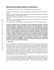
and a set of relevant possibly faulty system components (e.g. lines of code, gates in a circuit). The model includes descriptions of the interrelation between the components (e.g. wires between gates), descriptions of the components’ nominal behavior (e.g. relation between inputs and outputs of a gate) and other relevant knowledge (e.g. axioms of Boolean logic). An MBD problem arises if observations (e.g. sensor readings, system outputs) of the system’s behavior differ from predictions based on the system model. In this case, the set of observations is inconsistent with the system model under the assumption that all system components are exhibiting a nominal behavior. The sought solution to an MBD problem is a diagnosis pinpointing the faulty components causing the observed system failure. Normally, however, due to initially insufficient observations, this fault localization is ambiguous and multiple possible diagnoses exist. Sequential Diagnosis methods [de Kleer and Williams, 1987, Pietersma et al., 2005, Feldman et al., 2010, Siddiqi and Huang, 2011, Shchekotykhin et al., 2012] address this issue. These collect additional information by generating a sequence of queries and assume available some oracle providing answers to these queries. Depending on the MBD application domain, queries can be, for instance, measurements (e.g. probes in a circuit), system tests (observations about the system’s behavior upon new system inputs), questions to a domain expert (e.g. to a doctor when debugging a medical knowledge base) or component inspections (e.g. checking the battery of a car). Likewise, the instantiation of the oracle might be, for instance, an electrical engineer performing probes using a voltmeter, an IDE running software tests or a car mechanic inspecting components of a vehicle. If queries are chosen properly, each query’s answer eliminates some diagnoses and thus reduces the diagnostic uncertainty (pruning of the space of possible diagnoses). As query answering is normally costly, the goal of sequential diagnosis is to minimize the diagnostic cost in terms of, e.g., time, manpower or equipment required to achieve a diagnostic goal, e.g., the extraction of a diagnosis with a probability above some threshold or the isolation of a single remaining diagnosis (which then corresponds to the actual diagnosis, i.e. the actual cause of the system failure). A generic sequential diagnosis system is illustrated by Fig. 1. It gets the inputs SD (system description), COMPS (system components), OBS (initial observations), MEAS (additional observations / performed measurements), which altogether make up a diagnosis problem instance (DPI), and possibly some fault information (e.g. in terms of failure probabilities of system components). The usual workflow (see numbers in Fig. 1) followed by such a system involves the (1) computation of a (feasible) set of diagnoses by a diagnosis engine using the DPI and fault information, (2) computation of a set of query candidates by a query generation module based on the given diagnoses, (3) selection of the best query from the given candidates, (4) answering of this query by the interacting oracle, (5+6) addition of the returned query along with its answer to the DPI in terms of new measurements (MEAS). The diagnosis engine uses these new measurements to perform various updates (e.g. pruning of the diagnoses space, adapting the fault information). If the diagnostic goal is not accomplished, the entire process starts anew from (1). Otherwise, the best diagnosis is output. The focus of this work lies on the optimization of steps (2) and (3) in terms of both efficiency and output quality (see violet shaded area in Fig. 1). Note, the steps (1) and (2) draw on a logical reasoner. Since logical reasoning is one of the main sources of complexity in sequential diagnosis, the amount of reasoning should be ideally as minimal as possible, indicated by the red arrow in Fig. 1. Basically, there are two different rea2


Input: SD, COMPS, OBS, MEAS

SEQUENTIAL DIAGNOSIS SYSTEM 2: Queries

Query Generation

Query Selection

5: Query+Answer

DPI

3: Best Query

4: Answer

Oracle

1: Diagnoses 6: New Measurement(s) Input

Diagnosis Engine

Fault Information

Logical Reasoner

Output: Diagnosis D*

Figure 1: Schematic view on a generic sequential diagnosis system. The area shaded in violet shows the part of the system optimized by the approach in this work. The red arrow emphasizes that (expensive) reasoner calls have to be minimized.

soning paradigms sequential diagnosis systems might use, glass-box and black-box. Glass-box approaches directly integrate reasoning with diagnoses finding with the goal of achieving better performance. To this end the internals of the reasoner are suitably modified or, respectively, reasoners are complemented by additional services, e.g., bookkeeping in an ATMS [de Kleer, 1986]. One example [de Kleer and Williams, 1987] is the storing of (minimal) environments (sets of logical sentences sufficient) for entailments predicted by the system model. These are leveraged to compute so-called nogood sets [de Kleer, 1986], i.e. environments for entailments inconsistent with observations. The latter can be directly used for diagnoses construction. Glassbox approaches are therefore dependent on the particular (modified) reasoner and thus on the particular logic for which the reasoner is sound and complete. Black-box approaches use the reasoner as an oracle for answering consistency or entailment queries. The reasoner is used as-is without requiring any alterations to its implementation or any supplements. Consequently, these approaches are independent of the logic used for describing the system model and of the particular reasoner employed, and can benefit from latest improvements of reasoning algorithms. For instance, black-box approaches can switch to reasoners specialized in a certain sublanguage (e.g. polynomial-time reasoner ELK [Kazakov et al., 2014] for OWL EL [Krötzsch, 2010]) of a logic (e.g. OWL 2 [Grau et al., 2008] where reasoning is N2EXPTIME-complete) “for free” in a simple plug-in fashion if the system description is formalized in this sublanguage. First, while glass-box approaches in many cases offer some performance gain over blackbox approaches, this gain was shown to be not that significant – in most cases the time cost of both paradigms lay within the same order of magnitude – in extensive evaluations carried out by [Horridge, 2011] using Description Logics [Baader et al., 2007] of reasoning complexity ranging from polynomial to N2EXPTIME-complete. Black-box approaches even outperformed glass3

box approaches in a significant number of cases, witnessed in similar experiments conducted by [Kalyanpur, 2006]. When using bookkeeping methods, the information stored by these might grow exponentially with the problem size [Schiex and Verfaillie, 1994]. Moreover, switching to more efficient reasoners (e.g., for fragments of a logic, see above) is not (easily) possible for glass-box approaches. Second, system descriptions (SD) in MBD might use a wide range of different knowledge representation formalisms such as First-Order Logic fragments, Propositional Logic, Horn clauses, equations, constraints, Description Logics or OWL. For these reasons we present a logics- and reasoner-independent black-box approach to sequential diagnosis which is appropriate for all monotonic and decidable knowledge representation languages. This preserves a maximal generality of our approach and makes it broadly applicable across different MBD application domains. Because the problem of optimal query selection1 is NP-complete [Hyafil and Rivest, 1976], sequential diagnosis approaches have to bear on a trade-off between query optimality and computational complexity. Therefore, it is current practice to rely on myopic (usually one-step lookahead) methods to guide diagnoses discrimination [de Kleer and Williams, 1987, Feldman et al., 2010, Gonzalez-Sanchez et al., 2011, Shchekotykhin et al., 2012, Rodler et al., 2013]. Empirical [de Kleer et al., 1992b, Shchekotykhin et al., 2012, Rodler et al., 2013] and theoretical [Pattipati and Alexandridis, 1990] evaluations have evidenced that such heuristic methods in many cases deliver reasonable and in some scenarios even (nearly) optimal results. Moreover, query selection based on a multi-step lookahead is computationally prohibitive due to the involved expensive model-based reasoning (cf. Sec. 5). In common with the above-mentioned approaches we model the query selection heuristic as a query selection measure m assigning a real-value to each query based on its quality (regarding diagnoses discrimination). One popular such measure is entropy [de Kleer and Williams, 1987], which favors queries with a maximal expected information gain or, equivalently, a maximal expected reduction of the diagnostic uncertainty. The goal of any such measure m is the minimization of the number of queries required until achieving the appointed diagnostic goal. Whereas sequential diagnosis approaches usually incorporate the optimization of a query selection measure m, they often do not optimize the query (answering) cost such as the time required to perform measurements [Heckerman et al., 1995]. We model this cost by a query cost measure c, a function allocating a real-valued cost to each query. The approach suggested in this work is devised to compute optimized queries along the m and c axes at each (query selection) step in the sequential diagnosis process while minimizing the required computational resources. More concretely, the contributions of this work are the following: Contributions. We present a novel query optimization method that is generally applicable to any MBD problem in the sense of [de Kleer and Williams, 1987, Reiter, 1987] and 1. defines a query as a set of First-Order Logic sentences and thus generalizes the measurement notion of [de Kleer and Williams, 1987, Reiter, 1987], 2. given a set of leading diagnoses [de Kleer and Williams, 1989], allows the two-dimensional optimization of the next query in terms of the expected number of subsequent queries (measure m) and query cost (measure c), 1. Also known as Optimal Test Sequencing Problem [Pattipati and Alexandridis, 1990] or Optimal Decision Tree Problem [Hyafil and Rivest, 1976].

4


3. for an aptly refined (yet exponential) query search space, finds – without any reasoner calls – the globally optimal query w.r.t. measure c that globally optimizes measure m,2 4. for the full query search space, finds – with a polynomial number of reasoner calls – the (under reasonable assumptions) globally optimal query w.r.t. m that includes, if possible, only “cost-preferred” sentences (e.g. those answerable using built-in sensors), 5. guarantees the proposal of queries that discriminate between all leading diagnoses and that unambiguously identify the actual diagnosis. Furthermore, 6. we show that any MBD problem can be reduced to a Knowledge Base Debugging (KBD) problem [Shchekotykhin et al., 2012, Rodler, 2015]. This result establishes a formal relationship between these two paradigms, shows the greater generality of the latter and enables the transferral of findings in the KBD domain to the MBD domain. In a nutshell, the presented query optimization method can be subdivided into three phases, P1, P2 and P3. In the first place, P1 optimizes the next query’s discrimination properties (e.g. the expected information gain) based on the criteria imposed by the given QSM m, realized by a heuristic backtracking search. Then, as a first option, P2 computes an optimal query Q∗ regarding the given QCM c by running a uniform-cost hitting set tree search over a suitable (and explicitly given) set of partial leading diagnoses. This is done in a way Q∗ meets exactly the optimal discrimination properties determined in P1. P2 explores the largest possible query search space that can be handled without any reasoner calls in a complete way. The output Q∗ suggests the inspection of the system component(s) that is least expensive for the oracle (QCM c) among all those that yield the highest information (QSM m). As a second option and alternative to P2, P3 performs a two-step optimization consisting of a first generalization of the addressed search space and a subsequent divide-and-conquer exploration of this search space focused on cost-preferred measurements. P3 returns a cost-optimal query Q∗ (w.r.t. some QCM c) complying with the optimal discrimination properties fixed in P1. Q∗ may include measurements of arbitrary type, depending on priorly definable requirements. Roughly, the efficiency of the novel approach is possible by the recognition that the optimizations of m and c can be decoupled and by using logical monotonicity as well as the inherent (already inferred) information in the (⊆-minimal) leading diagnoses. The latter is leveraged to achieve a retention of costly reasoner calls until the final query computation stage (P3), and hence to reduce them to a minimum. In particular, the method is inexpensive as it (a) avoids the generation and examination of unnecessary (non-discriminating) or duplicate query candidates, (b) actually computes only the single best query by its ability to estimate a query’s quality without computing it, and (c) guarantees soundness and completeness w.r.t. an exponential query search space independently of the properties and output of a reasoner. 2. The term globally optimal has its standard meaning (cf. [Luenberger and Ye, 2015, p. 184]) and emphasizes that the optimum over all queries in the respective query search space is meant.

5

Modern sequential diagnosis methods like [de Kleer and Williams, 1987] and its derivatives [Feldman et al., 2010, Shchekotykhin et al., 2012, Rodler et al., 2013] do not meet all properties (a) – (c). The black-box approaches among them extensively call a reasoner in order to compute a query. As we show in our evaluations, the presented method can save an exponential overhead compared to these approaches. Moreover, we emphasize that our approach can also deal with problems where the query space is implicit, i.e. all possible system measurements cannot be enumerated in polynomial time in the size of the system model. E.g., in a digital circuit all measurement points (and hence the possible queries) are given explicitly by the circuit’s wires which can be directly extracted from the system description (SD). In, e.g., knowledge-based problems, by contrast, the possible measurements, i.e. questions to an expert, must be (expensively) inferred and are not efficiently enumerable. In fact, we show that for problems involving implicit queries, approaches not using the proposed theory might be drastically incomplete and hence might miss optimal queries. Finally, by the generality of our query notion, our method explores a more complex search space than [de Kleer and Williams, 1987, de Kleer and Raiman, 1993], thereby guaranteeing property (5) above. Organization. The rest of this work is organized as follows. Sec. 2 provides theoretical foundations needed in later sections. In particular, it gives a short introduction on Model-Based Diagnosis (MBD) in Sec. 2.1, on Knowledge Base Debugging (KBD) in Sec. 2.2 and formally proves that each MBD problem can be reduced to a KBD problem in Sec. 2.3. Henceforth, the work focuses w.l.o.g. just on KBD. Basics on Sequential Diagnosis including important definitions, the formal characterization of the addressed problem, and a generic algorithm to solve this problem are treated in Sec. 2.4. The main part of the paper starts with Sec. 3, where we first formalize the measurement selection problem (Sec. 3.1) and then discuss the proposed novel algorithm to solve this problem (Sec. 3.2). The presentation of our method is subdivided into a first part attempting to give the reader a prior intuition, motivation and overview of the later introduced theoretical concepts (Sec. 3.2.1), and three further parts, one dedicated to each phase (P1, P2 and P3) of the new algorithm (Sec. 3.2.2, 3.2.3 and 3.2.5). Besides an extensively exemplified expansion of the relevant theory, each phase description includes a complexity analysis. A formal specification of the computed solution’s properties for P1+P2 is given in Sec. 3.2.4 and for P3 in Sec. 3.2.6. Finally, Sec. 3.2.7 recapitulates the entire approach by means of a detailed example. Sec. 4 includes the description of our experimental evaluations in order to complement the theoretical findings of Sec. 3.2. The experimental settings are explicated in Sec. 4.1, whereas the experimental results are discussed in Sec. 4.2. Subsequently, there is a section on related work (Sec. 5) before we conclude with Sec. 6. Appendix A comprises all proofs that are not given in the text. Appendix B provides a table including all important symbols used in the text along with their meaning.

2. Preliminaries In this section, we revise the general theory of Model-Based Diagnosis (MBD) proposed by [Reiter, 1987], define the knowledge base debugging framework (KBD) we will use to formalize MBD problems in this work, and demonstrate that KBD is a generalization of MBD. 6


2.1 Model-Based Diagnosis We briefly review the classical model-based diagnosis (MBD) problem described by [Reiter, 1987]. At first, we characterize a system, e.g. a digital circuit, a car or some software, which is the subject of a diagnosis task: Definition 1 (System). A system is a tuple (SD, COMPS) where SD, the system description, is a set of First-Order Logic sentences, and COMPS, the system components, is a finite set of constants c1 , . . . , cn . The distinguished unary “abnormal” predicate AB is used in SD to model the expected behavior of components c ∈ COMPS. Let us denote the First-Order Logic sentence describing this expected behavior of c by beh(c) and let SDbeh := {¬AB(c) → beh(c) | c ∈ COMPS}. The latter subsumes a statement of the form “if c is nominal (not abnormal), then its behavior is beh(c)” for each system component c ∈ COMPS. Any behavior different from beh(c) implies that c is at fault, i.e. AB(c) holds. But, an abnormal component does not necessarily manifest a faulty behavior in each situation (weak fault model [de Kleer et al., 1992a, Feldman et al., 2009]), e.g. for an or-gate c stuck at 1 faulty behavior ¬beh(c) can only be observed if both inputs are 0. Further, SD might include general axioms describing the system domain or descriptions of the interplay between the system components. Let us call the set of these general axioms SDgen . So, SD = SD beh ∪ SD gen . The behavior of a system (SD, COMPS) assuming all components working correctly is captured by the description SD ∪ {¬AB(c) | c ∈ COMPS}. Note, this description is equal to SDgen ∪ {beh(c) | c ∈ COMPS}. A diagnosis problem arises when the observed system behavior – represented by a finite set of First-Order Logic sentences OBS – differs from the expected system behavior. Formally, this means that SD ∪ {¬AB(c) | c ∈ COMPS} ∪ OBS |= ⊥. For instance, in circuit diagnosis OBS might be the observation of the system inputs and outputs. There are usually multiple different hypotheses (diagnoses) that explain the discrepancy between observed and predicted system behavior. Discrimination between these hypotheses can then be accomplished by means of additional observations MEAS called measurements [Reiter, 1987, de Kleer and Williams, 1987]. Each measurement m in the set of measurements MEAS is a set of First-Order Logic sentences [Reiter, 1987] describing additional knowledge about the actual system behavior, e.g. whether a particular wire in a faulty circuit is high or low. Usually new measurements are conducted and added to MEAS until some diagnostic goal G is achieved, e.g. the presence of just a single or one highly probable remaining hypothesis. Each added measurement m, if chosen properly, will invalidate some hypotheses. Throughout this paper we assume stationary health [Feldman et al., 2010], i.e. that one and the same (faulty) behavior can be constantly reproduced for each c ∈ COMPS during system diagnosis. Formalized, these notions lead to the definitions of an MBD diagnosis problem instance (MBD-DPI) and of an MBD-diagnosis. Definition 2 (MBD-DPI). Let OBS (system observations) be a finite set of First-Order Logic sentences, MEAS (measurements) be a finite set including finite sets mi of First-Order Logic sentences, and let (SD, COMPS) be a system. Then the tuple (SD, COMPS, OBS, MEAS) is an MBD diagnosis problem instance (MBD-DPI). 7

Definition 3. Let DPI := (SD, COMPS, OBS, MEAS) be an MBD-DPI and UMEAS denote the union of all m ∈ MEAS. Then SD∗ [∆] := SD ∪{AB(c) | c ∈ ∆}∪{¬AB(c) | c ∈ COMPS \ ∆}∪ OBS ∪ UMEAS for ∆ ⊆ COMPS denotes the behavior description of the system ( SD, COMPS ) • under the current state of knowledge given by the DPI in terms of OBS and MEAS, and • under the assumption that all components in ∆ ⊆ COMPS are faulty and all components in COMPS \ ∆ are healthy. Definition 4 (MBD-Diagnosis). Let DPI := (SD, COMPS, OBS, MEAS) be an MBD-DPI. Then ∆ ⊆ COMPS is an MBD-diagnosis for DPI iff SD∗ [∆] is consistent (∆ explains OBS and MEAS). An MBD-diagnosis ∆ for DPI is called minimal iff there is no MBD-diagnosis ∆0 for DPI such that ∆0 ⊂ ∆. In many practical applications there are multiple (minimal) MBD-diagnoses for a given MBD-DPI. Without additional information about the system, one cannot conjecture a unique diagnosis. The idea is then to perform measurements in order to discriminate between competing (minimal) MBD-diagnoses until a sufficient degree of diagnostic certainty (the specified diagnostic goal G) is reached. This is the problem addressed by Sequential MBD and can be stated as follows: Problem 1 (Sequential MBD). . Given: An MBD-DPI DPI := (SD, COMPS, OBS, MEAS) and a diagnostic goal G. Find: MEASnew ⊇ ∅ and ∆, where MEASnew is a set of new measurements such that ∆ is a minimal MBD-diagnosis for the MBD-DPI DPInew := (SD, COMPS, OBS, MEAS ∪ MEASnew ) and ∆ satisfies G. Remark 1 Due to the intractability of the computation of the entire set of minimal diagnoses [Bylander et al., 1991], both the measurement selection and the decision whether a diagnostic goal G is satisfied for some diagnosis D is usually made by using a (computationally feasible) set of leading minimal diagnoses D [de Kleer and Williams, 1989]. D acts as an approximation of all minimal diagnoses for the given DPI and usually comprises the most probable minimal [de Kleer and Williams, 1989] or minimum-cardinality [Feldman et al., 2010] diagnoses for a DPI. Given a set of leading minimal diagnoses D for DPInew , examples for the specification of G are G1 := “D is the only minimal diagnosis for DPInew ” [de Kleer and Raiman, 1993], G2 := “D exceeds some predefined probability threshold t”, e.g. t := 0.95 [de Kleer and Williams, 1987, Shchekotykhin et al., 2012] or G3 := “D has ≥ k times the probability of all other elements in D”. Note that the goal G1 represents a maximally strict requirement on the final diagnostic result as it requires the verification of the invalidity of all but the correct minimal diagnosis (we call a diagnostic goal Gi more strict than a diagnostic goal Gj if Gj is satisfied earlier in any diagnostic session than Gi ). The specification of (constants in) G depends on the seriousness of misdiagnosis, e.g. higher probability thresholds signify higher criticality. In general, the size of the search space for minimal MBD-diagnoses for (SD, COMPS, OBS, is in O(2|COMPS| ). A useful concept to restrict this search space is the one of an MBDconflict [Reiter, 1987, de Kleer and Williams, 1987], a set of components whose elements cannot all be healthy given OBS and MEAS: MEAS)

8


X1

circuit inputs (from top to bottom) 1 0 1 circuit outputs (from top to bottom) 1 0

X2

A2

A1

O1

Figure 2: MBD Example due to [Reiter, 1987] from the domain of circuit diagnosis. Definition 5 (MBD-Conflict). Let DPI := (SD, COMPS, OBS, MEAS) be an MBD-DPI. Then C ⊆ COMPS is an MBD-conflict for DPI iff SD ∪{¬AB(c) | c ∈ C}∪ OBS ∪UMEAS is inconsistent. An MBD-conflict C for DPI is called minimal iff there is no MBD-conflict C 0 for DPI such that C 0 ⊂ C. Definition 6 (Hitting Set). Let S = {S1 , . . . , Sn } be a collection of sets. Then H is called a hitting set of S iff H ⊆ US and H ∩ Si 6= ∅ for all i = 1, . . . , n. A hitting set H of S is minimal iff there is no hitting set H 0 of S such that H 0 ⊂ H. The following result [Reiter, 1987] can be used to determine MBD-diagnoses through the computation of MBD-conflicts: Theorem 1. A (minimal) MBD-diagnosis for a DPI is a (minimal) hitting set of all minimal MBD-conflicts for this DPI. Example 1 Let us revisit the circuit diagnosis example given in [Reiter, 1987] shown in Fig. 2. The first step towards diagnosing the circuit using MBD is to formulate the problem as an MBDDPI. The result ExM := (SD, COMPS, OBS, MEAS) is given by Tab. 1 and explained next. The circuit, i.e. the system to be diagnosed, includes five gates X1 , X2 (xor-gates), A1 , A2 (and-gates) and O1 (or-gate), which are at the same time the system components COMPS of interest. The system description SD = SDbeh ∪ SDgen consists of a knowledge base SDbeh = {α1 , . . . , α5 } describing the behavior of each gate given it is working properly, e.g. for gate X1 , SDbeh includes the sentence α1 := (¬AB(X1 ) → out(X1 ) = xor(in1(X1 ), in2(X1 ))). Besides, SD includes a knowledge base SDgen = {α6 , . . . , α12 } describing which gate-terminals are connected by wires, e.g. the wire connecting X1 to X2 is defined by the sentence α7 := (out(X1 ) = in1(X2 )). For simplicity we omit the explicit statement of additional general domain knowledge in SDgen such as axioms for Boolean algebra or axioms restricting wires to only either 0 or 1 values. The observations OBS = {α13 , . . . , α17 } are given by the system inputs and outputs (see the table in Fig. 2). Finally, since there are no already performed measurements, the set MEAS is empty. Assuming all components are healthy, i.e. all gates function properly, we find out that SD∗ [∅] is inconsistent (cf. Def. 3). That is, the assumption of no faulty components conflicts with the observations OBS made. E.g., if X1 and X2 manifest nominal behavior, we can deduce that 9

the output out(X2 ) = 0 which contradicts the observation sentence α16 := (out(X2 ) = 1). Supposing either of the components X1 , X2 to be nominal, we can no longer deduce out(X2 ) = 0 (or any other sentence contradicting OBS). Therefore, C1 := {X1 , X2 } is a minimal MBDconflict (cf. Def. 5). Similarly, we find that C2 := {X1 , A2 , O1 } is the only other minimal MBD-conflict for ExM. Computing minimal hitting sets of all minimal MBD-conflicts C1 , C2 , we obtain three minimal MBD-diagnoses ∆1 := {X1 }, ∆2 := {X2 , A2 } and ∆3 := {X2 , O1 }. Let the diagnostic goal G be the achievement of complete diagnostic certainty, i.e. to single out the correct minimal MBD-diagnosis. The goal of the MBD-problem is then to find new measurements m1 , . . . , mk such that there is a single minimal diagnosis ∆ for (SD, COMPS, OBS, MEAS ∪ {m1 , . . . , mk }). Let the first measurement m1 be the observation of the terminal out(X1 ), and let the value of it be 0. Then, ∆1 is still a minimal MBD-diagnosis for ExMnew := (SD, COMPS, OBS, MEAS ∪ {{out(X1 ) = 0}}) since the abnormality of X1 explains both OBS and MEAS. Moreover, all other MBD-diagnoses for ExMnew must contain X1 (since its faultiness is the only explanation for MEAS) and thus be supersets of ∆1 . Hence, ∆1 is the only minimal MBD-diagnosis for ExMnew and thus the actually faulty component in this scenario is X1 (under the assumption that a ⊆-minimal set of components is broken). This fact could be derived by conducting only one measurement.

2.2 Knowledge Base Debugging In this section we revisit the knowledge base debugging (KBD) problem [Friedrich and Shchekotykhin, 2005, Shchekotykhin et al., 2012, Rodler, 2015] which we will use subsequently as a generalized reformulation of Reiter’s original MBD problem described above. Besides offering some notational conveniences, KBD allows users to specify negative measurements (or test cases) [Felfernig et al., 2004a]. Contrary to (positive) measurements m ∈ MEAS as characterized above, negative measurements state properties that must not hold. In other words, any diagnosis must fulfill that – under its assumption – the system description together with the observations and positive measurements does not entail any negative measurement. Additionally, it is possible in KBD to postulate stronger logical properties apart from consistency. For example, when debugging an ontology (i.e. a system where COMPS are ontology axioms) one might want the assumption of a diagnosis to yield a coherent [Schlobach et al., 2007, Parsia et al., 2005] system description (repaired ontology), i.e. one without unsatisfiable classes. In First-Order Logic terms (using logic programming notation), an unsatisfiable class in a KB K is an n-ary predicate r such that K |= ∀X ¬r(X) where X = X1 , . . . , Xn . That is, coherency means that every predicate in K can have some instance without yielding an inconsistency. Another possible use case for the adoption of (logical) requirements such as coherency is the fault localization in flawed (e.g. inconsistent) system models used for MBD. For instance, a model (which is itself a KB) used to describe the circuit in Fig. 2 might include an unsatisfiable class xor (which essentially makes the model inconsistent after the creation of, e.g., the sentence xor (X1 ) declaring X1 as an xor-gate). The reason for this incoherency might be that SDgen includes the sentences xor (G) → gate(G) and gate(G) → and (G) ∨ or (G) ∨ not(G) (where the system modeler forgot to include xor (G)) as well as sentences stating that no instance can 10


i 1 2 3 4 5 6 7 8 9 10 11 12 13 14 15 16 17

αi ¬AB(X1 ) → beh(X1 ) ¬AB(X2 ) → beh(X2 ) ¬AB(A1 ) → beh(A1 ) ¬AB(A2 ) → beh(A2 ) ¬AB(O1 ) → beh(O1 ) out(X1 ) = in2(A2 ) out(X1 ) = in1(X2 ) out(A2 ) = in1(O1 ) in1(A2 ) = in2(X2 ) in1(X1 ) = in1(A1 ) in2(X1 ) = in2(A1 ) out(A1 ) = in2(O1 ) in1(X1 ) = 1 in2(X1 ) = 0 in1(A2 ) = 1 out(X2 ) = 1 out(O1 ) = 0

SD beh

SD gen

i 1 2 3 4 5 6 7 8 9 10 11 12 13 14 15 16 17

OBS

• • • • • • • • • • • • • • • • •

COMPS

{X1 , X2 , A1 , A2 , O1 } c X1 X2 A1 A2 O1

beh(c) for c ∈ COMPS out(X1 ) = xor(in1(X1 ), in2(X1 )) out(X2 ) = xor(in1(X2 ), in2(X2 )) out(A1 ) = xor(in1(A1 ), in2(A1 )) out(A2 ) = xor(in1(A2 ), in2(A2 )) out(O1 ) = xor(in1(O1 ), in2(O1 ))

i ×

MEAS

αi out(X1 ) = xor(in1(X1 ), in2(X1 )) out(X2 ) = xor(in1(X2 ), in2(X2 )) out(A1 ) = and(in1(A1 ), in2(A1 )) out(A2 ) = and(in1(A2 ), in2(A2 )) out(O1 ) = or(in1(O1 ), in2(O1 )) out(X1 ) = in2(A2 ) out(X1 ) = in1(X2 ) out(A2 ) = in1(O1 ) in1(A2 ) = in2(X2 ) in1(X1 ) = in1(A1 ) in2(X1 ) = in2(A1 ) out(A1 ) = in2(O1 ) in1(X1 ) = 1 in2(X1 ) = 0 in1(A2 ) = 1 out(X2 ) = 1 out(O1 ) = 0

i ×

pi ∈ P ×

i ×

ni ∈ N ×

i 1

ri ∈ R consistency

K • • • • •

B

• • • • • • • • • • • •

min KBD-conflicts {α1 , α2 } , {α1 , α4 , α5 } min KBD-diagnoses {α1 } , {α2 , α4 } , {α2 , α5 }

×

Table 1: MBD-DPI ExM obtained from circuit diagnosis problem in Fig. 2.

Table 2: KBD-DPI ExM2K obtained from MBD-DPI ExM from Tab. 1.

be of more than one type of gate. That is, KBD (with the coherency requirement) could be used in such scenario to repair the model thus enabling a sound diagnostic process. 2.2.1 T HE U SED N OTATION Let L denote some formal knowledge representation language. We will call αL , α1,L , α2,L , . . . ∈ L logical sentences over L and a set of logical sentences KL ⊆ 2L a knowledge base (KB) over L. Sentences in KL will sometimes be referred to as axioms. We denote by |=L ⊆ 2L × L the semantic entailment relation for the logic L and we write KL |=L αL to state that αL is a logical consequence of the KB KL . For brevity, we will write K1,L |=L K2,L for two KBs K1,L and K2,L to denote that K1,L |=L αL for all αL ∈ K2,L and K1,L 6|=L αL to state that K1,L 6|=L αL for some αL ∈ K2,L . Given a collection of sets X, we use UX and IX to denote the union and intersection, respectively, of all elements in X. Further, Tab. 7 (see Appendix B) summarizes the meaning of other formalisms used in the paper (many of them introduced at some later point). 11

2.2.2 A SSUMPTIONS The KBD techniques described in this work are applicable to any knowledge representation formalism L which is Tarskian, i.e. for which the semantic entailment relation |=L is monotonic, idempotent and extensive [Tarski, 1983, Ribeiro, 2012] and for which reasoning procedures for deciding consistency of a KB over L are available. Definition 7. The relation |=L is called • monotonic iff whenever KL |=L αi,L then KL ∪ {αk,L } |=L αi,L (i.e. adding new sentences to a KB cannot invalidate any entailments of the KB) • idempotent iff KL |=L αi,L and KL ∪ {αi,L } |=L αk,L implies KL |=L αk,L (i.e. adding entailed sentences to a KB does not yield new entailments of the KB) • extensive iff KL |=L αL for all αL ∈ KL (i.e. each KB entails all sentences it comprises). In the following, “sentence” will always mean “logical sentence”. We will omit the index L for brevity when referring to sentences or KBs, tacitly assuming that any sentence or KB we speak of is formulated over some (fixed) language L where L meets the conditions given above. Examples of logics that comply with these requirements include, but are not restricted to Propositional Logic, Datalog [Ceri et al., 1989], (decidable fragments of) First-Order Predicate Logic, The Web Ontology Language (OWL [Patel-Schneider et al., 2004], OWL 2 [Grau et al., 2008, Motik et al., 2009]), sublanguages thereof such as the OWL 2 EL Profile (with polynomial time reasoning complexity [Kazakov et al., 2014]), Boolean or linear equations and various Description Logics [Baader et al., 2007] and constraint languages. 2.2.3 D EFINITIONS AND P ROPERTIES We next state the KBD problem and give some important definitions and properties (discussed in detail in [Rodler, 2015]). The inputs to a KB debugging problem can be characterized as follows: Given is a KB K to be repaired and a KB B (background knowledge). All sentences in B are considered correct and all sentences in K are considered potentially faulty. K∪B does not meet postulated requirements R (where consistency is a least requirement3 ) or does not feature desired semantic properties, called test cases. Positive test cases (aggregated in the set P ) correspond to necessary entailments and negative test cases (aggregated in the set N ) represent necessary non-entailments of the correct (repaired) KB (together with the background KB B). Each test case p ∈ P and n ∈ N is a set of sentences. The meaning of a positive test case p ∈ P is that the union of the repaired KB and B must entail each sentence (or the conjunction of sentences) in p, whereas a negative test case n ∈ N signalizes that some sentence (or the conjunction of sentences) in n must not be entailed by this union. The described inputs to the KB debugging problem are captured by the notion of a KBD diagnosis problem instance (KBD-DPI): 3. We assume consistency a minimal requirement to a solution KB provided by a debugging system, as inconsistency makes a KB completely useless from the semantic point of view.

12


i 1 2 3 4 5 6 7 8 9

αi ¬H ∨ ¬G X ∨F →H E → ¬M ∧ X A → ¬F K→E C→B M →C∧Z H→A ¬B ∨ K

K • • • • • • •

i 1

pi ∈ P {¬X → ¬Z}

i 1 2 3

ni ∈ N {M → A} {E → ¬G} {F → L}

i 1

ri ∈ R consistency

B

• •

min KBD-conflict X C1 C2 C3 C4

{i | αi ∈ X} {1, 2, 3} {2, 4} {2, 7} {3, 5, 6, 7}

explanation |= n2 ∪ {8} |= ¬F (|= n3 ) ∪ {p1 , 8} |= n1 ∪ {9} |= ¬M (|= n1 )

min KBD-diagnosis X D1 D2 D3 D4 D5 D6

{i | αi ∈ X} {2, 3} {2, 5} {2, 6} {2, 7} {1, 4, 7} {3, 4, 7}

explanation Theorem 3 Theorem 3 Theorem 3 Theorem 3 Theorem 3 Theorem 3

Table 4: Minimal KBD-conflicts and KBD-diagnoses for the KBD-DPI ExK in Tab. 3.

Table 3: Running example KBD-DPI ExK over Propositional Logic.

Definition 8 (KBD-DPI). Let • • • • •

K be a KB, P , N be sets including sets of sentences, R ⊇ {consistency} be a set of (logical) requirements, B be a KB such that K ∩ B = ∅ and B satisfies all requirements r ∈ R, and the cardinality of all sets K, B, P , N be finite.

Then we call the tuple hK, B, P , N iR a KBD diagnosis problem instance (KBD-DPI).

Example 2 An example ExK of a Propositional Logic KBD-DPI is depicted by Tab. 3. ExK will serve as a running example throughout this paper. It includes a KB K with seven axioms α1 , . . . , α7 , a background KB B with two axioms α8 , α9 , one singleton positive test case p1 and three singleton negative test cases n1 , n2 , n3 . There is one requirement r1 = consistency in R imposed on the correct (repaired) KB. It is easy to verify that the standalone KB B = {α8 , α9 } is consistent, i.e. satisfies all r ∈ R, and that K ∩ B = ∅. Hence, ExK indeed constitutes a KBD-DPI as per Def. 8. A solution (KB) for a DPI is characterized as follows:

13

Definition 9 (Solution KB). Let DPI := hK, B, P , N iR be a KBD-DPI. Then a KB K∗ is called solution KB w.r.t. DPI iff all the following conditions hold: ∀r ∈ R : ∀p ∈ P ∀n ∈ N

: :

K∗ ∪ B fulfills r

(1)

∗

(2)

∗

(3)

K ∪ B |= p K ∪ B 6|= n.

A solution KB K∗ w.r.t. DPI is called maximal iff there is no solution KB K0 w.r.t. DPI such that K0 ∩ K ⊃ K∗ ∩ K (i.e. K∗ has a set-maximal intersection with K among all solution KBs). Usually, observing the Principle of Parsimony [Reiter, 1987], maximal solution KBs K∗ will be preferred to non-maximal ones since they result from the input KB K through the modification of a minimal set of axioms. Example 3 For the KBD-DPI ExK given by Tab. 3, K = {α1 , . . . , α7 } is not a solution KB w.r.t. hK, B, P , N iR since, e.g. clearly K ∪ B = {α1 , . . . , α9 } 6|= p1 which is a positive test case and therefore has to be entailed. Another reason why K = {α1 , . . . , α7 } is not a solution KB w.r.t. ExK is that K ∪ B ⊃ {α1 , α2 , α3 } |= n2 , which is a negative test case and hence must not be an entailment. This is straightforward since {α1 , α2 , α3 } imply E → X, X → H and H → ¬G and thus clearly n2 = {E → ¬G}. On the other hand, Ka∗ := {}∪{Z → X} is clearly a solution KB w.r.t. ExK as {Z → X}∪B is obviously consistent (satisfies all r ∈ R), does entail p1 ∈ P and does not entail any ni ∈ N , (i ∈ {1, 2, 3}). However, Ka∗ is not a maximal solution KB since, e.g. α5 = (K → E) ∈ K can be added to Ka∗ without resulting in the violation of any of the Equations (1) – (3). Note that also e.g. {¬X → ¬Z, A1 → A2 , A2 → A3 , . . . , Ak−1 → Ak } for arbitrary finite k ≥ 0 is a solution KB, albeit not a maximal one, although it has no axioms in common with K and includes an arbitrary number of axioms not occurring in K. However, to maintain a maximum amount of the knowledge specified in the KB K of interest, one will usually prefer minimally invasive modifications (i.e. maximal solution KBs) while repairing faults in K. Maximal solution KBs w.r.t. the given DPI are, e.g. Kb∗ := {α1 , α4 , α5 , α6 , α7 , p1 } (resulting from the deletion of {α2 , α3 } from K and the addition of p1 ) or Kc∗ := {α1 , α2 , α5 , α6 , p1 } (resulting from the deletion of {α1 , α4 , α7 } from K and the addition of p1 ). That these KBs constitute solution KBs can be verified by checking the three conditions named by Def. 9. Indeed, adding an additional axiom in K to any of the two KBs leads to the entailment of a negative test case n ∈ N . That is, no solution KB can contain a proper superset of the axioms from K that are contained in any of the two solution KBs Kb∗ and Kc∗ . Hence, both are maximal. Remark 2 There are generally infinitely many (maximal) solution KBs resulting from the deletion of one and the same set of axioms D from the original KB K. This stems from the fact that there are infinitely many (semantically equivalent) syntactical variants of any set of suitable sentences that can be added to K \ D in order for Eq. (2) to be satisfied. One reason for this is that there are infinitely many tautologies that might be included in these sentences, another reason is that sentences can be equivalently rewritten, e.g. A → B ≡ A → B ∨ ¬A ≡ A → B ∨ ¬A ∨ ¬A ≡ . . . . 14


In terms of our running example, this circumstance can be illustrated as follows: Example 4 Consider again ExK in Tab. 3 and assume D = {α2 , α3 } is deleted from K. Then one solution KB constructible from K\D is Kb∗ given in the last example. To determine the maximal solution KB Kb∗ from K\D, the most straightforward way of adding just all sentences occurring in positive test cases in P has been chosen in this case. Other maximal solution KBs obtain∗ := {α , α , α , α , α , Z → X} (which difable from adding sentences to K \ D are, e.g. Kb1 1 4 5 6 7 ∗ := {α , α , α , α , α , Z → X ∧ W } fers syntactically, but not semantically from Kb∗ ) and Kb2 1 4 5 6 7 (which differs both syntactically and semantically from Kb∗ yielding the entailment Z → W which is not implied by Kb∗ ). Despite generally multiple semantically different solution KBs, the diagnostic evidence of a DPI in terms of positive test cases P does not justify the inclusion of sentences (semantically) different from UP (cf. [Friedrich and Shchekotykhin, 2005, Shchekotykhin et al., 2012]). Since we are moreover interested in only one instance of a solution KB resulting from K \ D for each D, we define K \ D ∪ UP as the canonical solution KB for D w.r.t. DPI iff K \ D ∪ UP is a solution KB w.r.t. DPI. A KBD-diagnosis is defined in terms of the axioms D that must be deleted from the KB K of a DPI in order to construct a solution KB w.r.t. this DPI. In particular, the deletion of D from K targets the fulfillment of Equations (1) and (3) such that UP can be added to the resulting modified KB K \ D without introducing any new violations of (1) or (3). Definition 10 (KBD-Diagnosis). Let DPI := hK, B, P , N iR be a KBD-DPI. A set of sentences D ⊆ K is called a KBD-diagnosis w.r.t. DPI iff (K \ D) ∪ UP is a solution KB w.r.t. DPI (i.e. K∗ := (K \ D) ∪ UP meets Equations (1) – (3)). A KBD-diagnosis D w.r.t. DPI is • minimal iff there is no D0 ⊂ D such that D0 is a KBD-diagnosis w.r.t. DPI • a minimum cardinality KBD-diagnosis w.r.t. DPI iff there is no KBD-diagnosis D0 w.r.t. DPI such that |D0 | < |D|. We will write D ∈ allDDPI to state that D is a KBD-diagnosis w.r.t. DPI and D ∈ minDDPI to state that D is a minimal KBD-diagnosis w.r.t. DPI. Remark 3 Since (K \ D) ∪ UP trivially satisfies (2) due to the inclusion of UP , D is a KBDdiagnosis w.r.t. DPI iff K∗ := (K \ D) ∪ UP satisfies (1) and (3). The next theorem captures the relationship between maximal canonical solution KBs and minimal KBD-diagnoses w.r.t. a DPI. In fact, it tells us that we can concentrate only on the computation of minimal KBD-diagnoses in order to find all maximal canonical solution KBs. Theorem 2. Let DPI := hK, B, P , N iR be a KBD-DPI. Then the set of all maximal canonical solution KBs w.r.t. DPI is given by {(K \ D) ∪ UP | D is a minimal KBD-diagnosis w.r.t. DPI}. In a completely analogous way as MBD-conflicts provide an effective mechanism for focusing the search for MBD-diagnoses, we can exploit KBD-conflicts for KBD-diagnoses calculation. Simply put, a (minimal) KBD-conflict is a (minimal) per se faulty subset of the original KB K, i.e. one source causing the faultiness of K in the context of B ∪ UP . For a KBD-conflict 15

there is no extension that yields a solution KB. Instead, such an extension is only possible after deleting appropriate axioms from the KBD-conflict. Definition 11 (KBD-Conflict). Let DPI := hK, B, P , N iR be a KBD-DPI. A set of formulas C ⊆ K is called a KBD-conflict w.r.t. DPI iff C ∪ UP is not a solution KB w.r.t. DPI (i.e. K∗ := C ∪ UP violates at least one of the Equations (1) – (3)). A KBD-conflict C w.r.t. DPI is minimal iff there is no C 0 ⊂ C such that C 0 is a KBD-conflict w.r.t. DPI. Theorem 3. [Friedrich and Shchekotykhin, 2005, Prop. 2] Let DPI be a KBD-DPI. Then a (minimal) KBD-diagnosis w.r.t. DPI is a (minimal) hitting set of all minimal conflicts w.r.t. DPI. Proposition 1. [Rodler, 2015, Prop. 3.4] Let DPI := hK, B, P , N iR be a KBD-DPI. Then a KBD-diagnosis w.r.t. DPI exists iff B ∪ UP satisfies all r ∈ R and B ∪ UP 6|= n for all n ∈ N . Example 5 Tab. 4 gives a list of all minimal KBD-conflicts w.r.t. our running example ExK. Let us briefly reflect why these are KBD-conflicts (cf. third col. of Tab. 4). Recall Ex. 3, where we explained why C1 is a KBD-conflict (violation of n2 ∈ N ). C1 is minimal since, first, it is consistent, i.e. satisfies all r ∈ R, and does not entail any of the negative test cases n1 , n3 . So, by logical monotonicity no proper subset of C1 can violate r, n1 or n3 . Second, the elimination of any axiom αi (i ∈ {1, 2, 3}) from C1 breaks the entailment of the negative test case n2 . Regarding C2 := {α2 , α4 }, we have that (any superset of) C2 is a KBD-conflict due to (the monotonicity of Propositional Logic and) the fact that α2 ≡ {X → H, F → H} together with α8 (∈ B) = H → A and α4 = A → ¬F clearly yields F → ¬F ≡ ¬F which, in particular, implies n3 = {F → L} ≡ {¬F ∨ L}. C3 is a minimal KBD-conflict since it is a ⊆-minimal subset of the KB K which, along with B and UP (in particular with α8 ∈ B and p1 ∈ P ), implies that n1 ∈ N must be true. To see this, realize that α7 |= M → Z, p1 = Z → X, α2 |= X → H and α8 = H → A, from which n1 = {M → A} follows in a straightforward way. Finally, C4 is a KBD-conflict since α7 |= M → C, α6 = C → B, α9 ≡ B → K, α5 = K → E and α3 |= E → ¬M . Again, it is now obvious that this chain yields the entailment ¬M which in turn entails {¬M ∨ A} ≡ {M → A} = n1 . Clearly, the removal of any axiom from this chain breaks the entailment ¬M . As this chain is neither inconsistent nor implies any negative test cases other than n1 , the conflict C4 is also minimal. It is not very hard to verify that there are no other minimal KBD-conflicts w.r.t. ExK apart from C1 , . . . , C4 . Example 6 The set minDExK of all minimal KBD-diagnoses w.r.t. ExK (Tab. 3) is shown in Tab. 4. Theorem 3 and the illustration (given in Ex. 5) of why C1 , . . . , C4 constitute a complete set of minimal KBD-conflicts w.r.t. ExK provide the explanation for minDExK . For instance, D1 = {α2 , α3 } “hits” the element α2 of Ci (i ∈ {1, 2, 3}) and the element α3 of C4 . Note also that it hits two elements of C1 which, however, is not necessarily an indication of the nonminimality of the hitting set. Indeed, if α2 is deleted from D1 , it has an empty intersection with C2 and C3 and, otherwise, if α3 is deleted from it, it becomes disjoint with C4 . Hence D1 is actually a minimal hitting set of all minimal KBD-conflicts. The relationship between the notions KBD-diagnosis, solution KB and KBD-conflict is as follows (cf. [Rodler, 2015, Cor. 3.3]): 16


Proposition 2. Let D ⊆ K. Then the following statements are equivalent: 1. D is a KBD-diagnosis w.r.t. hK, B, P , N iR . 2. (K \ D) ∪ UP is a solution KB w.r.t. hK, B, P , N iR . 3. (K \ D) is not a KBD-conflict w.r.t. hK, B, P , N iR . Example 7 Since, e.g., K \ D := {α1 , α2 } is not a KBD-conflict w.r.t. ExK (Tab. 3), we obtain that D = K\(K\D) = {α1 , . . . , α7 }\{α1 , α2 } = {α3 , . . . , α7 } is a KBD-diagnosis w.r.t. ExK, albeit not a minimal one (α5 and α6 can be deleted from it while preserving its KBD-diagnosis property). Further on, (K \ D) ∪ UP = {α1 , α2 , p1 } must be a solution KB w.r.t. ExK. 2.3 Reducing Reiter’s MBD Problem to KB Debugging We next demonstrate that the classical MBD problem described in Sec. 2.1 can be reduced to the KBD problem explicated in Sec. 2.2 [Rodler and Schekotihin, 2017]. That is, any MBD-DPI can be modeled as a KBD-DPI, and the solutions of the latter directly yield the solutions of the former. Theorem 4 (Reduction of MBD to KBD). Let mDPI := (SD, COMPS, OBS, MEAS) be an MBDDPI where COMPS = {c1 , . . . , cn }. Then, mDPI can be formulated as a KBD-DPI kDPI such that there is a bijective correspondence between KBD-diagnoses for kDPI and MBD-diagnoses for mDPI. Moreover, all MBD-diagnoses for mDPI can be computed from the KBD-diagnoses for kDPI. Proof. We first show how mDPI can be formulated as a KBD-DPI kDPI. To this end, we specify how kDPI = hK, B, P , N iR can be written in terms of the components of mDPI = (SDbeh ∪ SDgen , COMPS, OBS, MEAS): K = {αi | αi := beh(ci ), ci ∈ COMPS}

(4)

B = OBS ∪ SDgen

(5)

P = MEAS

(6)

N =∅

(7)

R = {consistency}

(8)

That is, K captures SDbeh ∪ {¬AB(ci ) | ci ∈ COMPS}, i.e. the nominal behavioral descriptions of all system components. By Def. 10 and Remark 3, D ⊆ K is a KBD-diagnosis for kDPI iff (K \ D) ∪ B ∪ UP satisfies all r ∈ R

(i.e. is consistent)

(9)

and (K \ D) ∪ B ∪ UP 6|= n for all n ∈ N

(10)

Let now D be an arbitrary KBD-diagnosis for kDPI such that D = {αi | i ∈ I} for the index set I ⊆ {1, . . . , n}. 17

Using (4) – (8) above, condition (9) for D is equivalent to the consistency of SDbeh ∪{AB(ci ) | i ∈ I} ∪ {¬AB(ci ) | i ∈ {1, . . . , n} \ I} ∪ OBS ∪ SDgen ∪ UMEAS which in turn yields that SD

∪ {AB(ci ) | ci ∈ ∆} ∪ {¬AB(ci ) | ci ∈ COMPS \ ∆} ∪ OBS ∪ UMEAS is consistent

(11)

for ∆ := {ci | ci ∈ COMPS, i ∈ I}. But, (11) is exactly the condition defining an MBDdiagnosis (see Def. 4). Note, since N = ∅ by (7), condition (10) is satisfied for any D satisfying (9) and can thus be neglected. Hence, D = {αi | i ∈ I} ⊆ K is a KBD-diagnosis w.r.t. kDPI iff ∆ = {ci | ci ∈ COMPS, i ∈ I} ⊆ COMPS is an MBD-diagnosis for mDPI. Also, there is a bijective correspondence between KBD-conflicts and MBD-conflicts: Proposition 3. Let mDPI = (SD, COMPS, OBS, MEAS) be an MBD-DPI and kDPI = hK, B, P , N iR a KBD-DPI modeling mDPI as per (4) – (8). Further, let COMPS = {c1 , . . . , cn } and I ⊆ {1, . . . , n}. Then, C = {ci | ci ∈ COMPS, i ∈ I} ⊆ COMPS is an MBD-conflict for mDPI iff C = {αi | i ∈ I} ⊆ K is a KBD-conflict w.r.t. kDPI. Proof. C is a KBD-conflict w.r.t. kDPI iff K \ C = {αi | i ∈ {1, . . . , n} \ I} is not a KBDdiagnosis w.r.t. kDPI (Prop. 2) iff {ci | ci ∈ COMPS, i ∈ {1, . . . , n} \ I} is not an MBD-diagnosis for mDPI (Theorem 4) iff {ci | ci ∈ COMPS, i ∈ I} = C is an MBD-conflict for mDPI ([Reiter, 1987, Prop. 4.2]). Let us exemplify these theoretical results: Example 8 Reconsider the circuit diagnosis example (Fig. 2). The formalization of the circuit problem as an MBD-DPI ExM was discussed in Ex. 1. The formulation of this MBD-DPI as a KBD-DPI ExM2K as per Eq. (4) – (8) is depicted by Tab. 2. All minimal KBD-conflicts and their minimal hitting sets, i.e. the minimal KBD-diagnoses (Theorem 3), are given in the lower part of Tab. 2. For instance, C = {α1 , α4 , α5 } is a KBD-conflict w.r.t. ExM2K since C ∪ B ∪ UP |= ⊥. We briefly sketch why this holds. α13 (∈ B) = (in1(X1 ) = 1), α14 (∈ B) = (in2(X1 ) = 0) and α1 = (out(X1 ) = xor (in1(X1 ), in2(X1 ))) imply that out(X1 ) = xor (1, 0) = 1, which, along with α6 (∈ B) = (out(X1 ) = in2(A2 )), entails in2(A2 ) = 1, which in turn, together with α15 (∈ B) = (in1(A2 ) = 1) and α4 = (out(A2 ) = and (in1(A2 ), in2(A2 ))), lets us deduce that out(A2 ) = and (1, 1) = 1. Because of α8 (∈ B) = (out(A2 ) = in1(O1 )) we have that in1(O1 ) = 1 which yields out(O1 ) = or (1, in2(O1 )) = 1 due to α5 = (out(O1 ) = or (in1(O1 ), in2(O1 ))). However, α17 ∈ B states that out(O1 ) = 0, a contradiction. C is minimal since all elements of C were necessary to derive the outlined contradiction. In fact, no proper subset of C can be used to deduce any negative test case (trivially, as the set N is empty) or any contradiction (possibly different from the one given above). Intuitively, the latter holds since any C 0 ⊂ C includes too few behavioral descriptions of components so that there is no “open” path for constraint propagation from inputs to outputs of the circuit. C, on the other hand, enables to propagate information from all three inputs via gates X1 , A2 and O1 towards the second output. What becomes nicely evident at this point is the principle of transformation between MBD and KBD. Whereas in MBD behavioral descriptions of components are “disabled” via abnormality assumptions about components, in KBD it is exactly these descriptions that make up the KB, and they are “inactivated” by just deleting them from the KB. 18


The justification for the minimal KBD-conflict {α1 , α2 } follows essentially the same argumentation as was given in Ex. 1 to explain C1 . To sum up, we can find all diagnoses for any MBD-DPI by representing it as a KBD-DPI and solving the KBD-DPI (Theorem 4). Thus, KBD methods [Shchekotykhin et al., 2012, Rodler, 2015] are suitable for MBD as well. Moreover, computing all minimal diagnoses for KBD-DPIs leads us to all maximal (canonical) solution KBs w.r.t. the DPI in a trivial way (Theorem 2). Due to these results we can henceforth w.l.o.g. restrict our focus to KBD problems and the computation of minimal diagnoses w.r.t. these problems. However, we bear in mind that the presented methods apply to MBD problems as well and the obtained solutions can be easily reformulated as solutions for knowledge-based system debugging. Hence, whenever we will write DPI, diagnosis and conflict in the rest of this work, we will refer to KBD-DPI, KBD-diagnosis and KBD-conflict, respectively. The problem of Sequential Diagnosis, which will generalize the Sequential MBD-Problem as per Prob. 1, will be discussed in detail in the next section. 2.4 Sequential Diagnosis Given multiple diagnoses for a DPI, sequential diagnosis techniques [de Kleer and Williams, 1987, Brodie et al., 2003, Feldman et al., 2010, Siddiqi and Huang, 2011, Rodler et al., 2013, Shchekotykhin et al., 2014, Rodler, 2015] target the acquisition of additional information to minimize the diagnostic uncertainty, i.e. to reach a predefined diagnostic goal G (cf. Remark 1 for some examples). Depending on the sequential diagnosis framework, different types of information might be incorporated. For example, the framework used by [Brodie et al., 2003, Shchekotykhin et al., 2016] tests (sets of) components directly and takes the information about their normal/abnormal state into account. On the other hand, the approaches of [de Kleer and Williams, 1987, Siddiqi and Huang, 2011] indirectly measure values of variables influenced by the normal/abnormal behavior of components. As opposed to these probing techniques, testing approaches [Pattipati and Alexandridis, 1990, Shakeri et al., 2000, Feldman et al., 2010] observe particular system outputs after varying particular system inputs, i.e. the gathered information in this paradigm corresponds to input-output vectors. Our approach uses a way of information representation that, in principle, allows to model all aforementioned paradigms (see Ex. 9). Namely, we define a proposed measurement generally as a set of sentences (over some logic complying with the criteria given in Sec. 2.2.2), according to [Reiter, 1987]. We call a proposed measurement a query [Settles, 2012] if the additional information it gives eliminates in any case at least one (known) diagnosis [Shchekotykhin et al., 2012, Rodler, 2015]. Further on, we assume an entity, called oracle, capable of performing the required measurements. That is, an oracle answers queries by assessing the correctness of the sentences in the query. When diagnosing physical systems [de Kleer and Williams, 1987, Reiter, 1987, Heckerman et al., 1995], the oracle might be constituted by a human operator or automatic sensors making observations. For instance, when diagnosing a car, a car mechanic might act as an oracle. During the diagnosis of knowledge-based systems [Rodler, 2015] such as configuration systems [Felfernig et al., 2004a] or ontologies [Shchekotykhin et al., 2012], 19

the oracle could be a domain expert or some automatic information extraction system providing domain-specific knowledge. Given a query Q = {α1V , . . . , αk } containing the sentences4 α1 , . . . , αk , posing Q to the oracle means asking whether ki=1 αi must be true, or equivalently, whether each single sentence αi ∈ Q must be true. Hence, a query is answered by true (t) if the performed measurements confirm all sentences in Q, and by false if the measurements disprove some sentence(s) in Q. Depending on the concrete diagnosis task at hand, queries are answered w.r.t. different reference points. For instance, in the KB debugging domain, the desired model of the domain of interest, i.e. the correct KB, is the relevant reference point. That is, measurements in this case might correspond to cognitive activity (of a domain expert thinking about the truth of the sentences in Q) or the process of information extraction (of e.g. some system browsing some knowledge source relevant to Q). On the other hand, when diagnosing some physical device, the reference point is constituted by the actual behavior of the device. In this case a measurement is the observation of some system aspect(s) relevant to Q. So, given a reference point Ref , a positive answer to the query Q means that Ref |= Q, a negative one that Ref 6|= Q. In the sequential diagnosis process, the information provided by answered queries is incorporated into the current DPI, yielding a new (updated) DPI. In particular, a positively answered query Q is added as a positive test case to the current DPI hK, B, P , N iR resulting in the new DPI hK, B, P ∪ {Q} , N iR . Likewise, a negatively answered query Q is added as a negative test case to the current DPI hK, B, P , N iR resulting in the new DPI hK, B, P , N ∪ {Q}iR . In this vein, the successive addition of new answered queries to the test cases gradually reduces the diagnostic uncertainty by restricting the set of diagnoses. Note, if an oracle is able to provide any additional information, sentence(s) Y , beyond the mere query answer, e.g., an explanation or justification for a negative query answer, the presented approach enables to integrate and exploit this information for the invalidation of further diagnoses. To this end, Y is simply added to the set P as a positive test case. 2.4.1 D EFINITIONS AND P ROPERTIES We now present the concept of a query in more formal terms. In the following, given a DPI DPI := hK, B, P , N iR and some minimal diagnosis Di w.r.t. DPI, we will use the following abbreviation for the canonical solution KB obtained by deletion of Di along with the given background knowledge B: Ki∗ := (K \ Di ) ∪ B ∪ UP

(12)

4. We could also w.l.o.g. define a query to be a single logical sentence because it is interpreted as the conjunction of the sentences it contains, which is simply a “bigger” sentence. For technical reasons, we stick to the representation as a set of sentences (cf. [Reiter, 1987]), since we will present query minimization approaches for reducing the number of sentences in the query. This would correspond to reducing the length or complexity of the sentence in the single sentence interpretation of a query.

20


Proposition 4. Let DPI := hK, B, P , N iR be a DPI, X be a set of sentences and D ⊆ + − 0 minDDPI . Then X induces a partition PD (X) := D (X), D (X), D (X) on D where5 D+ (X) := {Di ∈ D | Ki∗ |= X} D− (X) := {Di ∈ D | (∃n ∈ N : Ki∗ ∪ X |= n) ∨ (∃r ∈ R : Ki∗ ∪ X violates r)} D0 (X) := D \ (D+ (X) ∪ D− (X)) Since the computation of all (minimal) diagnoses is computationally prohibitive in general, we exploit a subset D of all minimal diagnoses w.r.t. a DPI for measurement selection. D is referred to as the leading diagnoses (cf. Rem. 1). From a query we postulate two properties. It must for any outcome (1) invalidate at least one (leading) diagnosis (search space restriction) and (2) preserve the validity of at least one (leading) diagnosis (solution preservation). In fact, the sets D+ (X) and D− (X) are the key in deciding whether a set of sentences X is a query or not. Based on Prop. 4, we define: Definition 12 (Query, q-Partition). Let DPI := hK, B, P , N iR be a DPI, hK,B,P ,N i R

+D ⊆ minD be the leading diagnoses and Q be a set of sentences with PD (Q) = D (Q), D− (Q), D0 (Q) . Then Q is a query w.r.t. D iff Q 6= ∅, D+ (Q) 6= ∅ and D− (Q) 6= ∅. We denote the set of all queries w.r.t. D by QD . Further, we refer to the set of those Q ∈ QD with D0 (Q) = ∅ by QA0D . PD (Q) is called the q-partition of Q (or: a q-partition) iff Q is a query. Inversely, Q is called a query with (or: for) the q-partition PD (Q). Given a q-partition P, we sometimes denote its three entries in turn by D+ (P), D− (P) and D0 (P).6 Given the formal definition of a query, the oracle is formally defined as function ans : QD → {t, f } which outputs an answer ans(Q) for Q ∈ QD . D+ (Q) and D− (Q) denote those diagnoses in D consistent only with Q’s positive and negative outcome, respectively, and D0 (Q) those consistent with both outcomes. In other words, given the prior DPI DPI := hK, B, P , N iR and leading diagnoses D ⊆ minDDPI , then the posterior still valid diagnoses from D w.r.t. hK, B, P ∪ {Q} , N iR (i.e. after adding Q to the positive test cases) are those in D+ (Q) ∪ D0 (Q). The posterior still valid subset of D w.r.t. hK, B, P , N ∪ {Q}iR (i.e. after adding Q to the negative test cases) is D− (Q)∪D0 (Q). We also say that diagnoses in D+ (Q) predict Q’s positive answer, those in D− (Q) predict Q’s negative answer, and those in D0 (Q) do not predict any of Q’s answers. Since Q ∈ QD (Def. 12) implies that both D+ (Q) and D− (Q) are non-empty, clearly Q’s outcomes both dismiss and preserve at least one diagnosis, as postulated. Of course, in many cases a query will also invalidate some (unknown) non-leading diagnoses in allDDPI \ D. In fact, each query Q ∈ QD is necessarily also a query w.r.t. all minimal diagnoses, i.e. Q ∈ QminDDPI , and a query w.r.t. all diagnoses, i.e. Q ∈ QallDDPI . However, there might be sets of sentences X ∈ / QD which are in fact queries w.r.t. a different (e.g. a 0 larger) set of leading diagnoses D 6= D, i.e. X ∈ QD0 . Still, we point out that, facing the general intractability of the computation of multiple diagnoses, the best we can do is using the 5. We will often say “X violates R or N ” to state that (∃n ∈ N : X |= n) ∨ (∃r ∈ R : X violates r). 6. In existing literature, e.g. [Shchekotykhin et al., 2012, Rodler et al., 2013, Shchekotykhin and Friedrich, 2010], a q-partition is often simply referred to as partition. We call it q-partition to emphasize that not each partition of D into three sets is necessarily a q-partition.

21

currently given evidence in terms of the leading diagnoses D to differentiate between queries Q ∈ QD (definitely discriminating among all diagnoses) and non-queries Q0 ∈ / QD (potentially non-discriminating among all diagnoses). As the set D0 (Q) comprises those diagnoses that cannot be eliminated given any of Q’s outcomes, queries with non-empty D0 (Q) have a weaker discrimination power than others. The reason is that they discriminate only among the (leading) diagnoses D \ D0 (Q). Therefore, one will usually try to focus on queries with a set D0 (Q) as minimal in size as possible.7 In fact, [Rodler, 2015, p. 107 ff.] shows that it is always possible to enforce queries with empty D0 (Q) by making the comprised sentences sufficiently strong (in logical terms). Our new method presented in Sec. 3 guarantees the computation of only Q’s with D0 (Q) = ∅. On the one hand, this involves a focus on the promising query candidates (in that better discrimination among leading diagnoses lets us expect better discrimination among all diagnoses). On the other hand, it reduces the query (or more precisely: the q-partition) search space from O(3|D| ) (all 3-partitions of |D| diagnoses) to O(2|D| ) (all 3-partitions of D with one of the 3 sets, i.e. D0 , being empty). For example, the methods of [de Kleer and Williams, 1987, Shchekotykhin et al., 2012, Rodler et al., 2013] do not ensure these properties. Example 9 Consider the electronic circuit in Fig. 2. We exemplify how queries consisting of (e.g. First-Order Logic) sentences can be used to model direct (component) probing, indirect probing and testing. Direct Probing: A query representing a direct test of a component, say X1 , would be represented as Q = {beh(X1 )} = {out(X1 ) = xor (in1(X1 ), in2(X1 ))} (cf. Tab. 1 and Tab. 2), i.e. “Does component X1 work as expected?”. Such a direct test of a component might, depending on the application, involve visible, tangible or audible inspection, component examination using specialized tools, a check of operation logs for the component, etc. For instance, given a car that does not start, a direct component probe could involve testing whether the battery is working or dead using a battery test device. Indirect Probing: An indirect test of gates X1 and A1 could be formulated as a query Q = {out(A2 ) = 1}. The reason why these two gates are implicitly tested by answering Q is that these are the only gates influencing whether the tested wire between A2 and O1 is high or low (cf. Fig. 2). Note, if Q is answered negatively, this tells us that at least one component among {X1 , A2 } is defective. But if Q is positively answered, this gives us no definite information about the state of any of the two components (weak fault model). That is, both could be nominal, any 7. In fact, one can construct examples where a query Q with D0 (Q) 6= ∅ is better (w.r.t. to some query goodness measure m) than another one, Q0 , with D0 (Q0 ) = ∅. E.g., let m be the entropy measure [de Kleer and Williams,

1987] and p be a probability measure, then one such example is Q with p(D+ (Q)), p(D− (Q)), p(D0 (Q)) =

0 + 0 − 0 0 0 h0.49, 0.49, 0.02i and Q with p(D (Q )), p(D (Q )), p(D (Q )) = h0.99, 0.01, 0i. Nevertheless, first, in practice, given that Q is in QD , the existence of a query Q00 ∈ QD with small |p(D+ (Q00 )) − p(D+ (Q))| and small |p(D− (Q00 )) − p(D− (Q))| as well as p(D0 (Q00 )) = 0 is likely (e.g. by making Q logically stronger, cf. [Rodler, 2015, Chap. 8]). Second, we need to compare the best query with empty D0 with the best query with non-empty D0 (as we will present a search that finds the best query among those with empty D0 ). Except for very small search spaces (where brute force methods considering all queries are anyway practical), a query like Q0 will most probably not be the best query with empty D0 . Third, the query space |QD | is normally large enough to ensure the existence of (even multiple) very close-to-optimal queries as per some measure m even though those with non-empty D0 are neglected (cf. Sec. 4).

22


single one could be flawed, e.g. stuck-at-1, or both could be abnormal, e.g. X1 stuck-at-0 and A2 stuck-at-1. In the car example, an indirect test of the battery charge (and possibly some other components) could involve a test of the car’s ignition. Testing: Let us say we want to acquire diagnostic information by experimenting with various inputs and observing the resulting outputs of the circuit. A query testing whether the desired output (0, 0) results from the given input (0, 0, 0), would be of the form Q = {(in1(X1 ) = 0 ∧ in2(X1 ) = 0 ∧ in1(A2 ) = 0) → (out(X2 ) = 0 ∧ out(O1 ) = 0)}. Example 10 Let us consider our running example DPI ExK = hK, B, P , N iR (Tab. 3) let us further suppose that some diagnosis computation algorithm provides the set of leading diagnoses D = {D1 , D2 , D3 , D4 } (see Tab. 4). Then Q1 := {M → B} is a query w.r.t. D, i.e. Q1 ∈ QD . To verify this, we use Def. 12 directly and show that both D+ (Q1 ) 6= ∅ and D− (Q1 ) 6= ∅. We first consider the leading diagnosis D4 = {α2 , α7 } ∈ D. As per Eq. (12), we build the solution KB (with background knowledge) resulting from the application of D4 as K4∗ := (K \ D4 ) ∪ B ∪ UP . Since this KB does not entail Q1 (as can be easily verified using Tab. 3 and Tab. 4), D4 ∈ / D+ (Q1 ) (cf. D+ (X) in Prop. 4). So, we check whether D4 is an ele− ment of D (Q1 ). To this end, we first build K4∗ ∪ Q1 := (K \ D4 ) ∪ B ∪ UP ∪ Q1 = {α1 , α3 , α4 , α5 , α6 , α8 , α9 , p1 , M → B}. As α9 ≡ B → K, α5 = K → E and α3 |= E → ¬M , it is clear that {M → A} = n1 ∈ N is an entailment of K4∗ ∪ Q1 . Hence, D4 ∈ D− (Q1 ) (cf. D− (X) in Prop. 4) which is why D− (Q1 ) 6= ∅. Now, we have a look at D2 = {α2 , α5 }. We have that K2∗ := (K \ D2 ) ∪ B ∪ UP = {α1 , α3 , α4 , α6 , α7 , α8 , α9 , p1 } |= {M → B} = Q1 due to α7 |= M → C and α6 = C → B. Therefore, D2 ∈ D+ (Q1 ) which is why D+ (Q1 ) 6= ∅. All in all, we have proven that Q1 ∈ QD . If we complete the assignment to sets in the q-partition for all Di ∈ D, we obtain the qpartition PD (Q1 ) = h{D1 , D2 } , {D3 , D4 } , ∅i. The justification for the assignment of D1 and D3 is a follows. As K1∗ includes α6 , α7 we can conclude in an analogous way as above that K1∗ |= Q1 . In the case of D3 , we observe that K3∗ ∪ Q1 includes α3 , α5 , M → B and α9 . As explicated above, these axioms entail n1 ∈ N . The q-partition PD (Q1 ) indicates that D1 , D2 are invalidated given the oracle answers Q1 negatively, i.e. D1 , D2 ∈ / minDhK,B,P ,N ∪{Q1 }iR . Conversely, D3 , D4 are ruled out given Q1 ’s positive answer, i.e. D3 , D4 ∈ / minDhK,B,P ∪{Q1 },N iR . Some important properties of q-partitions and their relationship to queries are summarized by the next proposition: Proposition 5. [Rodler, 2015, Sec. 7.3 – 7.6] Let DPI := hK, B, P , N iR be a DPI and D ⊆ minDDPI . Further, let Q ∈ QD . Then: 1. hD+ (Q), D− (Q), D0 (Q)i is a partition of D. 2. D− (Q) contains exactly those diagnoses Di ∈ D where Di is not a diagnosis w.r.t. hK, B, P ∪ {Q} , N iR . D+ (Q) contains exactly those diagnoses Di ∈ D where Di is not a diagnosis w.r.t. hK, B, P , N ∪ {Q}iR . D0 (Q) contains exactly those diagnoses Di ∈ D where Di is a diagnosis w.r.t. both hK, B, P ∪ {Q} , N iR and hK, B, P , N ∪ {Q}iR . 3. For Q there is one and only one q-partition hD+ (Q), D− (Q), D0 (Q)i. 23

4. Q is a set of common entailments of all KBs in {Ki∗ | Di ∈ D+ (Q)}. That is, letting DC (X) denote the deductive closure of a set of sentences X, Q is a subset of the intersection of all DC (Ki∗ ) where Di used to construct Ki∗ is an element of D+ (Q). 5. A set of sentences X 6= ∅ is a query w.r.t. D iff D+ (X) 6= ∅ and D− (X) 6= ∅. 6. For each q-partition PD (Q) = hD+ (Q), D− (Q), D0 (Q)i it holds that D+ (Q) 6= ∅ and D− (Q) 6= ∅. 7. If |D| ≥ 2, then (a) Q := UD \ Di is a query w.r.t. D for all Di ∈ D, (b) h{Di } , D \ {Di } , ∅i is the q-partition associated with Q, and (c) a lower bound for the number of queries w.r.t. D is |D|. 2.4.2 T HE S EQUENTIAL D IAGNOSIS P ROBLEM The Sequential Diagnosis Problem we consider next is similar to the Sequential MBD-Problem (Prob. 1). The difference is that the former generalizes the latter by assuming an oracle that is allowed to not only specify positive test cases (cf. MEAS in Sec. 2.2.3) but also negative ones in order to narrow down the set of possible diagnoses. Problem 2 (Sequential Diagnosis). . Given: A DPI DPI := hK, B, P , N iR and a diagnostic goal G. Find: Pnew , Nnew ⊇ ∅ and D, where Pnew , Nnew are sets of positive and negative test cases, respectively, such that D is a minimal diagnosis w.r.t. DPInew := hK, B, P ∪ Pnew , N ∪ Nnew iR and D satisfies G. A generic algorithm solving this problem is given next. 2.4.3 A G ENERIC S EQUENTIAL D IAGNOSIS A LGORITHM The overall sequential diagnosis algorithm we take as a basis is described by Alg. 1. Similar algorithms are used e.g. in [de Kleer and Raiman, 1993, Shchekotykhin et al., 2012, Rodler, 2015]. Next, we briefly comment on the inputs, the output and the various steps of the algorithm (referred to by their line number in Alg. 1). (Inputs): The algorithm gets a DPI DPI and a diagnostic goal G as inputs (cf. Prob. 2). Further on, we assume some probability measure p that can be used to compute fault probabilities of sentences αi ∈ K and of diagnoses D ⊆ K. That is, we regard p as (i) a function p : K → [0, 1] assigning to each axiom in K (or: component in COMPS) a fault probability and (ii) a function p : allDDPI → [0, 1] mapping each diagnosis D w.r.t. DPI to its probability p(D). The latter is interpreted as the probability that all axioms in D are faulty and all axioms in K \ D are correct. In the circuit example of Fig. 2 and other physical devices, p might result from known or estimated fault probabilities of components (e.g. obtained from the component manufacturer or by observation) and other heuristic or experiential information [de Kleer and Kurien, 2004]. In a knowledge-based application, p might result from (an integration of) information about e.g. 24


common logical fault patterns [Roussey et al., 2009], logs of previous faults recorded by KB editors such as Protégé [Noy et al., 2000] or WebProtégé [Tudorache et al., 2011], user fault probabilities regarding syntactical [Shchekotykhin et al., 2012] or ontological [Rodler, 2015] elements in the KB, possibly coupled with provenance information about the KB’s sentences [Kalyanpur et al., 2006]. [Rodler, 2015, Sec. 4.6] provides a detailed discussion of applicable information sources for p and a derivation of diagnoses fault probabilities from axiom (or: component) fault probabilities or other sources. Hence, one can w.l.o.g. provide Alg. 1 only with axiom fault probabilities, i.e. the function in (i) above. Because the function in (ii) can be derived from the one in (i). Lastly, the algorithm is provided with a query quality measure qqm which enables the comparison of queries in QD and thus the determination of a favorable next query in each iteration. (Line 2): As a first step, the function COMPUTE L EADING D IAGNOSES computes a set of leading diagnoses D ⊆ minDDPI where |D| ≥ 2 if |minDDPI | ≥ 2. D usually comprises a number of most probable (by exploiting p) or minimum-cardinality diagnoses. To this end, several algorithms might be employed such as HS-T REE [Reiter, 1987] (possibly coupled with a minimal-conflict searcher, e.g. Q UICK X PLAIN [Junker, 2004], M ERGE X PLAIN [Shchekotykhin et al., 2015] or P ROGRESSION [Marques-Silva et al., 2013]), STATIC HS or DYNAMIC HS [Rodler, 2015], HS-DAG [Greiner et al., 1989], I NV-HS-T REE [Shchekotykhin et al., 2014] or Boolean algorithms [Jiang and Lin, 2003, Pill and Quaritsch, 2012]. The computed number |D| of leading diagnoses might be, e.g., predefined to some constant k [de Kleer and Raiman, 1993, Shchekotykhin et al., 2012], dependent on desired minimal and maximal bounds or computation time [Rodler, 2015], or a function of the probability measure p [de Kleer and Williams, 1989]. (Line 3): Then, the algorithm tests (usually by means of p, cf. Remark 1) whether the diagnostic goal G is satisfied for D. If so, the must probable leading diagnosis is returned (line 4) and the algorithm stops. (Line 5): Otherwise, the function CALC Q UERY determines a query Q by means of D, DPI, p and the qqm. Roughly, Q should discriminate optimally among minDDPI , or more precisely, among the leading diagnoses D, which is the currently available evidence regarding minDDPI . The meaning of “discriminating optimally” is determined by qqm which possibly relies upon p. That is, a query with best (or sufficiently good [de Kleer and Williams, 1987]) value as per qqm is sought among the queries in QD . One example of a qqm is the information-entropy-based $(.) function suggested by [de Kleer and Williams, 1987]. (Line 6): The calculated query is presented to the oracle and an answer ans(Q) is returned. This is the (only) point in the algorithm where an oracle inquiry takes place. For technical reasons, the oracle function ans is regarded as a total function, i.e. the oracle is assumed to be able to answer any posed query. We emphasize however that this is not a necessary requirement for our presented method which can handle do not know answers (e.g. if some measurement points in a physical device are not accessible to a technician) as well by simply offering the oracle the next-best query. Hence, one can imagine a (not shown) loop between lines 5 and 6 of the algorithm. (Line 7): Given the query-answer pair (Q, ans(Q)), the current DPI is updated by a respective addition of Q to the positive test cases P (i.e. P ← P ∪ {Q}) if ans(Q) = t and to N (i.e. N ← N ∪ {Q}) in case ans(Q) = f . Moreover, the function UPDATE DPI involves an adap25

tation of the diagnoses probability measure based on ans(Q) in terms of a Bayesian probability update according to [de Kleer and Williams, 1987, Shchekotykhin et al., 2012]. That is, for Q’s answer aQ ∈ {t, f } the new probability of any D ∈ allDDPI is computed as p(D | ans(Q) = aQ ) =

p(ans(Q) = aQ | D) p(D) p(ans(Q) = aQ )

The probabilities required to evaluate the above-notedP formula are established as follows. Given the current leading diagnoses D, we define p(X) := D∈X p(D) for X ⊆ D and assume p to be normalized over D such that that p(D) = 1. Since D includes only still possible diagnoses, p(D) > 0 must hold for all D ∈ D. Further, assuming that each non-predicting diagnosis D ∈ D0 (Q) predicts each answer with a probability of 12 , we define p(D0 (Q)) (13) 2 (i.e. the probability of the leading diagnoses predicting Q’s positive answer plus half the probability of the non-predicting leading diagnoses) and p(ans(Q) = f ) = 1 − p(ans(Q) = t) (i.e. the probability of the leading diagnoses predicting Q’s negative answer plus half the probability of the non-predicting leading diagnoses). Finally,  +  1, if D ∈ D (Q) p(ans(Q) = t | D) := 0, if D ∈ D− (Q)  1 0 2 , if D ∈ D (Q) p(ans(Q) = t) := p(D+ (Q)) +

and p(ans(Q) = f | D) = 1 − p(ans(Q) = t | D). Remark 4 When Alg. 1 computes a new set of leading diagnoses Dnew (line 2) after executing the DPI update in line 7, it computes Dnew as minimal diagnoses w.r.t. the new DPI. That is, D will usually (but not necessarily always, cf. [Rodler, 2015, Rem. 12.6]) comprise the remaining diagnoses from the leading diagnoses D used in the previous iteration and some new ones computed in line 2. The remaining diagnoses from D given ans(Q) = aQ are D+ (Q) ∪ D0 (Q) for aQ = t and D− (Q) ∪ D0 (Q) for aQ = f (cf. Prop. 5.2). (Outputs): The algorithm executes the while-loop until the given diagnostic goal G is fulfilled. Let DPI∗ be the current DPI and D be the current leading diagnoses in the iteration where this holds. Then Alg. 1 returns the most probable minimal diagnosis D∗ ∈ D ⊆ minDDPI∗ . 2.4.4 A LGORITHM C ORRECTNESS To show that Alg. 1 solves the Sequential Diagnosis problem (Prob. 2), we use the fact that for any non-singleton set of leading diagnoses D a query – and hence the opportunity to discriminate among elements of D – exists [Rodler, 2015, Sec. 7.6]: Proposition 6. Let DPI be a DPI and D ⊆ minDDPI such that |D| ≥ 2. Then QD 6= ∅. Theorem 5. Let COMPUTE L EADING D IAGNOSES be a sound and complete procedure for the computation of minimal diagnoses w.r.t. a DPI, CALC Q UERY be a sound method for query computation that returns at least one query for any D where QD 6= ∅, and G be an arbitrary 26


Algorithm 1 Sequential Diagnosis Input: DPI DPI := hK, B, P , N iR , diagnostic goal G, probability measure p (used to compute sentence and diagnoses fault probabilities), query quality measure qqm Output: The most probable minimal diagnosis D∗ ∈ D ⊆ minDDPI∗ where DPI∗ is some DPI hK, B, P 0 , N 0 iR where P 0 ⊇ P and N 0 ⊇ N such that the diagnostic goal G is met for D 1: while true do 2: D ← COMPUTE L EADING D IAGNOSES(DPI, p) 3: if GOAL R EACHED(G, D, p) then 4: return GET M OST P ROBABLE D IAGNOSIS(D, p) 5: Q ← CALC Q UERY(D, DPI, p, qqm) . see Algorithm 2 6: answer ← ans(Q) . oracle inquiry 7: DPI ← UPDATE DPI(DPI, p, Q, answer)

diagnostic goal that is at most as strict as G1 in Rem. 1. Then, for arbitrary inputs DPI (DPI), p (diagnoses probability measure) and qqm (query quality measure), Alg. 1 solves Prob. 2. Proof. (Sketch) Let us assume that G := G1 (“there is only a single minimal diagnosis w.r.t. the current DPI”) from Rem. 1 and let us refer to the DPI used by Alg. 1 in iteration i (of the while-loop) by DPIi , i.e. the input DPI DPI is denoted by DPI1 . If the first call of COMPUTE L EADING D IAGNOSES returns a singleton D = {D}, then |minDDPI | = 1, thus G1 is met and Alg. 1 returns D in line 4 which obviously meets Prob. 2 (Pnew = Nnew = ∅). Otherwise, the first call of COMPUTE L EADING D IAGNOSES returns some D where |D| ≥ 2. If G is not satisfied in line 3, then CALC Q UERY will return a query Q by Prop. 6. Due to [Rodler, 2015, Cor. 12.4], each answer ans(Q) implies that allDDPI1 ⊃ allDDPI2 where DPI2 is the result of applying UPDATE DPI in line 7 to DPI1 . We can now adopt the same argumentation for the second and any further call of COM PUTE L EADING D IAGNOSES (iterations 2, 3, . . . ). However, |allDDPI1 | must be finite as each diagnosis is a subset of K and K must be finite due to Def. 8. Hence, there must be some finite k such that G is met in line 3 of iteration k. Therefore, Alg. 1 outputs the single minimal diagnosis D w.r.t. DPIk which meets Prob. 2 (Pnew includes all the k1 positively answered queries in these k iterations, and Nnew all the k − k1 negatively answered ones). Since any diagnostic measure G Alg. 1 might be used with is at most as strict (cf. Rem. 1) as G1 , which we used for our argumentations, we obtain that such a finite k must always exist. 2.4.5 A PPLICABILITY AND D IAGNOSTIC ACCURACY Prop. 6 and Theorem 5 have two further implications: First, a precomputation of only two minimal diagnoses is required in each iteration to generate a query and proceed with sequential diagnosis. Despite its NP-hardness, the generation of two (or more) minimal diagnoses is practical in many real-world settings [de Kleer, 1991, Shchekotykhin et al., 2014], making query-based sequential diagnosis commonly applicable. Second, the query-based approach guarantees perfect diagnostic accuracy, i.e. the unambiguous identification of the actual diagnosis (e.g. by using the diagnostic goal G := G1 in Alg. 1). 27

3. Efficient Optimized Query Selection for Sequential Model-Based Diagnosis In this section we present the main contribution of this work, which is a novel implementation of the CALC Q UERY function in Alg. 1. But first, we have a look at the measurement selection problem in sequential diagnosis. 3.1 Measurement Selection for Sequential Diagnosis As argued, the (q-)partition PD (Q) enables both the verification whether a candidate Q is indeed a query and an estimation of the impact Q’s outcomes have in terms of diagnoses invalidation. And, given axiom (or: component) fault probabilities, it enables to gauge the probability of observing a positive or negative query outcome. Active learning query selection measures (QSMs) m : Q 7→ m(Q) ∈ R [Settles, 2012] use exactly these query properties characterized by the qpartition to assess how favorable a query is. They aim at selecting queries such that the expected number of queries until obtaining a deterministic diagnostic result is minimized, i.e. X p(D)q# (D) → min (14) D⊆K

where q# (D) is the number of queries required, given the initial DPI, to derive that D must be the actual diagnosis. Solving this problem is known to be NP-complete as it amounts to optimal binary decision tree construction [Hyafil and Rivest, 1976]. Hence, as it is common practice in sequential diagnosis [de Kleer and Williams, 1987, Brodie et al., 2003, Pietersma et al., 2005, Shchekotykhin et al., 2012, Rodler et al., 2013], we restrict our algorithm to the usage of QSMs that make a locally optimal query selection through a one-step lookahead. This has been shown to be optimal in many cases and nearly optimal in most cases [de Kleer et al., 1992b]. Several different QSMs m such as split-in-half, entropy, or risk-optimization have been proposed, well studied and compared against each other [de Kleer and Williams, 1987, Shchekotykhin et al., 2012, Rodler et al., 2013, Rodler, 2017]. For instance, using entropy as QSM, m would be exactly the scoring function $() derived in [de Kleer and Williams, 1987]. Note, we assume w.l.o.g. that the optimal query w.r.t. any m is the one with minimal m(Q). Besides minimizing the number of queries in a diagnostic session (Eq. (14)), a further goal can be the minimization of the query (answering) cost arising for the oracle. For instance, assume a malfunctioning physical system such as a car or a turbine. Then there might be parts of the system which are easier accessible, cheaper (in terms of required tools, time or manpower), less dangerous, etc. for measurements than others. In a car, it is clearly much easier and faster to check some, say cable, that is directly accessible after opening the engine cover than some internals of the engine. Apart from that, systems might include built-in sensors able to provide information about certain parts of the system quasi for free, whereas other parts must be manually measured. On the other hand, e.g., in knowledge-based systems, there might be sentences about the intended domain that are easier to evaluate than others. For example, sentences comprising complex logical notation are certainly more difficult to read, understand and thus to answer than, e.g., facts or simple implications (cf. [Ceraso and Provitera, 1971, Horridge et al., 2011]). Moreover, aside from the syntax of sentences, the comprehension of their content in terms of the expressed topic, can be a smaller or larger hurdle, depending on the oracle’s 28


expertise in the topic. E.g., given a faulty biomedical KB [Noy et al., 2009], a biologist acting as an oracle might be much less confident in answering a medicine-specific query than a biology-specific one. To this end, we allow the user of our tool to specify a query cost measure (QCM) c : Q 7→ c(Q) ∈ R+ that assigns to each query a real-valued cost. Examples of QCMs are P • cΣ (Q) := ki=1 ci (minimize overall query cost) • cmax (Q) := maxi∈{1,...,k} ci (minimize maximal cost of single measurements) • c|·| (Q) := |Q| (minimize number of measurements) where Q = {q1 , . . . , qk } and ci is the cost of evaluating the truth of the sentence qi . For example, the QCM cΣ could be used to minimize query answering time given that the ci ’s represent measurement time. Alternatively, cmax could be adopted, e.g., when the ci ’s account for human cognitive load, in order to keep the necessary cognitive skill to answer the query minimal. In scenarios where all potential measurements are known or assumed to be (approximately) equally costly to answer, one might pursue queries with a minimal number of sentences, which would be reflected by using the QCM c|·| . An example would be a digital circuit where all components and wires, respectively, are equally well accessible for measurements. Note that the QCM c|·| is a special case of cΣ , i.e. cΣ simulates c|·| if ci = cj for all i, j. In the following, we assume w.l.o.g. that the optimal query w.r.t. any c is the one with minimal c(Q). While the costs ci (e.g. accessibility of systems parts) relevant for physical systems might be more or less directly derivable from the structure or other properties of the system, the costs ci (e.g. comprehensibility of sentences) relevant for knowledge-based systems might be plausibly derivable from the available fault information [Rodler, 2015, Sec. 4.6.1]. For instance, the cognitive complexity of understanding a queried sentence correctly in terms of syntax and topic can be expected to be closely related to the fault probability of the sentence computed from fault information about logical elements (e.g. ∀, ¬, ∧) and non-logical elements (e.g. concepts such as toxoplasmosis or odontalgia in a medical KB). Intuitively, the more a sentence captures the expertise of the oracle (i.e. the lower its fault probability for the oracle is), the easier it is to understand and answer for the oracle. 3.1.1 T HE A DDRESSED M EASUREMENT S ELECTION P ROBLEM Now, the problem tackled by the new algorithm introduced in this work is: Problem 3 (Optimal Query Selection). . Given: A DPI DPI, D ⊆ minDDPI where |D| ≥ 2, a QSM m, a QCM c, a query search space S ⊆ QD . Find: A query Q∗ with minimal cost w.r.t. c among all queries in S that are optimal w.r.t. m. Formally: Q∗ = arg minQ∈OptQ(m,S) c(Q) where OptQ(m, S) := {Q0 | Q0 = arg minQ∈S m(Q)}. Note, there can be multiple equally good solutions Q∗ ∈ QD to Prob. 3. 3.2 The Suggested Algorithm In this section we propose a novel algorithm (Alg. 2) for two-way optimized query computation in sequential diagnosis which solves Prob. 3 (for different settings of the query search space 29

Algorithm 2 Optimized Query Computation Input: DPI DPI, D ⊆ minDDPI where |D| ≥ 2, a QSM m, a QCM c (including information about sentence costs ci , cf. page 29), probability measure p (to compute axiom fault probabilities), threshold tm (i.e. |m(Q) − mopt | ≤ tm ⇒ Q regarded as optimal; mopt := optimal value of m), inference engine Inf , set ET of entailment types, pref (preference information used for query optimization), a Boolean enhance (if true, optional query enhancement is run) Output: an optimized query Q∗ ∈ QD w.r.t. m, tm and c (cf. Theorems 7 and 8) 1: P ← OPTIMIZE QPARTITION(D, p, m, tm ) . P1 2: if enhance = true then 3: Q0 ← EXPAND Q UERY F OR QPARTITION(DPI, P, ET, Inf ) . (optional) P3 4: Q∗ ← OPTI M INIMIZE Q UERY F OR QPARTITION(DPI, P, Q0 , pref , Inf ) . (optional) P3 5: else 6: Q∗ ← OPTIMIZE Q UERY F OR QPARTITION(P, c) . (default) P2 7: return Q∗

S).8 The described query computation procedure can be divided into three phases: Phase P1 (line 1), (the default) Phase P2 (line 6) and (the optional) Phase P3 (lines 3-4). After giving the reader an intuition and overview of its functioning, we explain all three phases of it. Further implementation details can be found in the extended version [Rodler, 2016] of the paper. 3.2.1 I NTUITION AND OVERVIEW The main idea to achieve an inexpensive high-quality query generation is the exploitation of the information inherent in the ⊆-minimal leading diagnoses and a decoupling of the optimizations of a QSM (first), i.e. the minimization of the expected number of queries until diagnostic certainty is given, and a QCM (second), i.e. the minimization of the query (answering) costs. Phase P1, given a QSM m, determines an optimal QP w.r.t. m (which implies that all queries having this QP are optimal regarding m) by completely avoiding the use of reasoning services. For this purpose, we present a polynomial-space (heuristic) search technique that explores a generally exponential space of q-partitions in a sound and complete way. That is, without expensive reasoner calls, all non-QPs are automatically neglected (i.e. no unnecessary time is spent for exploring non-QPs) and the proven optimal QP in the explored space is found. As the key to the realization of this search, we introduce the notions of canonical queries and canonical QPs. Additionally, the use of these two concepts in phase P1 automatically disregards a broad class of suboptimal QPs, which leads to a generally significant refinement of the relevant search space. After an optimal QP P as per m has been determined and fixed, there are two options (parameter enhance): The execution of either • phase P2 (restricted search space, no reasoner calls, instantaneous output) or • phase P3 (full search space, polynomial number of reasoner calls, reasonably fast output). Phase P2 (enhance = false) realizes the finding of an optimal query w.r.t. any of the QCMs discussed on page 29 for the optimal QP P from P1. In order to make this query computation 8. A Protégé plugin for KB debugging implementing i.a. the presented algorithm can be found on http://isbi.aau.at/ontodebug/. Protégé [Noy et al., 2000] is the most widely used open-source KB (ontology) editor in the world and available at https://protege.stanford.edu/.

30


very efficient, P2 focuses on a restricted class of queries wherein the calculation of a (globally) optimal query is possible without reasoning aid. The query output by P2 represents the system component(s) whose inspection is least expensive (QCM c) among all those that yield the highest information (QSM m). In this vein, P2 computes an optimized query for scenarios such as the ones discussed in [Brodie et al., 2003]. Phase P3 (enhance = true) performs a query enhancement, subdivided into two consecutive steps. The first step “enriches” the canonical query of the optimal QP P from P1 by additional sentences of preferred types (augmentation to the full search space regarding preferred queries). The second step finds an optimized ⊆-minimal contraction of the enriched canonical query (searching for an optimal solution in full search space). Overall, phase P3 computes a query that globally optimizes the QCM cmax (see page 29) among all queries that – under the reasonable assumption given by Conjecture 1 (see later) – globally optimize the QSM m over the full query search space. To this end, P3 requires only a polynomial number of reasoner calls. Moreover, given any predefined set of preferred query elements (e.g. measurements with small costs), P3 ensures that the returned optimized query includes only such preferred elements, if such a query exists. 3.2.2 P HASE P1: O PTIMIZING THE Q-PARTITION In this section we describe the functioning of OPTIMIZE QPARTITION in Alg. 2. At this first stage P1, we optimize the given QSM m – for now without regard to the QCM c, which is optimized later in phase P2. This decoupling of optimization steps is possible since the QSM value m(Q) of a query Q is only affected by the (unique) q-partition of Q and not by Q itself. On the contrary, the QCM value c(Q) is a function of (the sentences in) Q only and not of Q’s q-partition. Therefore, the search performed in P1 will consider only q-partitions and target the determination of a (close-to) optimal q-partition P. This q-partition remains fixed throughout all further phases of the algorithm, where an optimal query with exactly this q-partition P is sought. Remark 5 A decoupling of optimizations in the reverse order, i.e. QCM c before QSM m, is not reasonably possible. First, the q-partition is a necessary prerequisite for the verification whether a set of sentences is in fact a query (see Def. 12). Because without the associated (q-)partition one has no guiding principle of which Q is allowed (i.e. a query) and which is not (i.e. a set of sentences that is not a query) when trying to find some query Q with minimal c(Q). Second, once the query is fixed, so is its q-partition (see Prop. 5.3). So, there is no chance to optimize m for some already fixed query Q. Canonical Queries and Q-Partitions. As the determination of an optimal q-partition w.r.t. the given QSM m should be as efficient as possible, we want to neglect any partition which is not a q-partition in the search. That is, we do not even want to generate any non-q-partitions. However, to verify whether a given 3-partition P of a set of leading diagnoses D is a q-partition, we need a query Q 6= ∅ with a q-partition PD (Q) = P. Q can be seen as a concrete witness proving that P is not solely a partition of D, but indeed a q-partition (cf. Def. 12). But:

31

Proposition 7. Let P be a (fixed) q-partition. Then |{Q | Q query, PD (Q) = P}| > 1, i.e. there are multiple queries for P. Proof. Since a query is a non-empty set of sentences, it must include at least one sentence α. This sentence can be equivalently rewritten in different ways, e.g. α ≡ α ∧ τ for an arbitrary tautology τ . Whereas the proof draws on a semantically equivalent rewriting (that is possible for any sentence in infinitely many ways) to show Prop. 7, we point out that there are, in most cases, queries with equal q-partitions that are semantically non-equivalent – and not even rewritings of one another. This holds true also for ⊆-minimal queries. i.e. queries where the removal of any sentence in them leads to a change of their associated q-partition. We will provide some examples later. The idea is now to appoint one well-defined representative query for each q-partition, i.e. we seek the definition of a unique query for each q-partition such that the former allows us to verify the latter. And, we want such a query to be easily computable. Furthermore, in order to devise a time and space saving q-partition search method, the potential size of the explored search space should to be minimized. To achieve this, a key idea is to omit those q-partitions in the search that are proven suboptimal. One such class of suboptimal q-partitions are those P with non-empty D0 (P) because they do not discriminate among all (leading) diagnoses (cf. the discussion in Sec. 2.4.1). Hence, a second postulation to the representative queries for q-partitions is that the focus on such queries implies the exclusion of the mentioned suboptimal q-partitions. In other words, each suboptimal q-partition should have no such representative query. To realize these postulations, we introduce the notion of a canonical query (CQ). The requirement of easy computability means that we would like to be able to determine a CQ without performing any expensive or (generally) intractable operations. Since by Prop. 4.4 any query

for a q-partition D+ , D− , D0 is a subset of the common entailments of all KBs in the set {Ki∗ | Di ∈ D+ }, the operations of interest in query computation are entailment calculations. Once calls to a reasoning engine are involved, the complexity of one such call is already NPcomplete for Propositional Logic. However, a straightforward way of entailment calculation without involving reasoning aid or other expensive operations is the restriction to the computation of explicit entailments. An entailment α of a KB X is called explicit iff α ∈ X, implicit otherwise [Rodler, 2015, Def. 8.1]. But, as indicated by [Rodler, 2015, Prop. 8.3], just these explicit entailments are also the key to achieve a disregard of suboptimal q-partitions. Therefore, CQs should be characterized as queries including only explicit entailments. Henceforth, we call a query Q ∈ QD explicit-entailments query iff Q ⊆ K. Indeed, a restriction to the consideration of only explicit-entailments queries leads to a focus on non-suboptimal q-partitions: Proposition 8. Let DPI := hK, B, P , N iR be a DPI, D ⊆ minDDPI and Q a query in QD such that Q ⊆ K. Then D0 (Q) = ∅. Proof. We have to show that for an arbitrary diagnosis Di ∈ D either Di ∈ D+ (Q) or Di ∈ D− (Q). Therefore two cases must be considered: (a) K \ Di ⊇ Q and (b) K \ Di 6⊇ Q. In case (a), by the fact that the entailment relation is extensive for L, K \ Di |= Q and thus, by 32


monotonicity of L, Ki∗ = (K \ Di ) ∪ B ∪ UP |= Q. So, Di ∈ D+ (Q). In case (b) there exists some axiom α ∈ Q ⊆ K such that α ∈ / K \ Di , which means that (K \ Di ) ∪ Q ⊃ (K \ Di ). From this we can derive that Ki∗ ∪ Q must violate R or N by the ⊆-minimality property of each diagnosis in D, in particular of Di . Hence, Di ∈ D− (Q). The proof of Prop. 8 exhibits a decisive advantage of using explicit-entailments queries. In fact, it reveals that the task of verifying whether a set of explicit entailments is a query in QD is very easy in that it can be reduced to set comparisons. That is, subset checks are traded for reasoning. To build the q-partition P(Q) associated with some explicit-entailments query Q it must solely be tested for each Di ∈ D whether K \ Di ⊇ Q or not. More specifically: Proposition 9. Let DPI := hK, B, P , N iR be a DPI, D ⊆ minDDPI and Q be a query in QD such that Q ⊆ K. Then D ∈ D+ (Q) iff K \ D ⊇ Q and D ∈ D− (Q) iff K \ D 6⊇ Q. The next proposition describes the shape any explicit-entailments query must have: Proposition 10. Let DPI be any DPI, D ⊆ minDDPI and Q be a query in QD such that Q ⊆ K. Then Q must include some axiom(s) in UD (i.e. Q ∩ UD 6= ∅), can but need not include any axioms in K \ UD , and must not include any axioms in ID (i.e. Q ∩ ID = ∅). Further on, elimination of axioms in K \ UD from Q does not affect the q-partition P(Q) of Q. As suggested by Prop. 10, the sentences in the KB K of a DPI that are crucial for the definition of an explicit-entailments query – and hence for the characterization of a CQ – are given by UD as well as ID . In fact, as the proofs of Lemmata 1 and 2 in Appendix A show, the noninclusion of sentences from ID is necessary to allow for non-empty D+ (Q) and the inclusion of some sentence(s) from UD is required to allow for non-empty D− (Q). Without these properties a set of sentences Q does not discriminate among the leading diagnoses D. For this reason, we give these essential sentences UD \ ID a distinct name: Definition 13. We call DiscD := UD \ ID the discrimination sentences wrt. D. Example 11 Let us consider the set of leading diagnoses D = {D1 , D2 , D3 } = {{α2 , α3 }, {α2 , α5 }, {α2 , α6 }}

(cf. Tab. 4)

w.r.t. our running example DPI ExK (Tab. 3). Then, UD = {α2 , α3 , α5 , α6 } and ID = {α2 }. Now, all ⊆-minimal explicit-entailments query candidates we might build according to Prop. 10 (which provides necessary criteria to explicit-entailments queries) are {{α3 , α5 , α6 } , {α3 , α5 } , {α3 , α6 } , {α5 , α6 } , {α3 } , {α5 } , {α6 }}

(15)

That is, all these seven candidates include at least one element out of UD and no elements out of K \ UD = {α1 , α4 , α7 } or ID . Clearly, there are exactly six different q-partition candidates with empty D0 w.r.t. the three diagnoses in D, i.e. there are three possibilities to select one, and three + + − possibilities to select two diagnoses to constitute D with ∅ ⊂ D ⊂ D (the set D

+ − the0set + is already set after D is chosen since D , D , D is a partition of D). Hence, QD might comprise at most six explicit-entailments queries with different q-partitions because each one of them must feature an empty D0 -set in its q-partition, as stated by Prop. 8. By the Pigeonhole 33

Principle, either at least two candidates in Eq. (15) have the same q-partition or at least one candidate is not a query at all. As we require that there must be exactly one CQ per q-partition and seek a method that computes only queries (and no candidates that turn out to be no queries), we see that Prop. 10 is not yet restrictive enough to constitute also a sufficient criterion for CQs. So let us now find out where the black sheep among the candidates above is. The key to finding it is the fact that each query Q is a common entailment of all Ki∗ := (K \ Di ) ∪ B ∪ UP where Di is in the D+ (Q)-set of Q’s q-partition (cf. Prop. 5.4). Since the candidates for CQs in Eq. (15) are all constituted of just explicit entailments αi ∈ K, we immediately see that we must postulate that each CQ Q is a set of common elements of all K \ Di where Di is in the D+ (Q)-set of Q’s q-partition. The K\Di sets for diagnoses Di ∈ D are given below. Starting to verify this for the first candidate {α3 , α5 , αT 6 } above, we quickly find out that there is no possible + D (Q)-set of a q-partition such that Q ⊆ Di ∈D+ (Q) K \ Di because none of these intersected sets includes all elements out of {α3 , α5 , α6 }. Thus, the first candidate is no query at all. K \ D1 = {α1 , α4 , α5 , α6 , α7 } K \ D2 = {α1 , α3 , α4 , α6 , α7 } K \ D3 = {α1 , α3 , α4 , α5 , α7 } Performing an analogue verification for the other candidates, we recognize that all of them are indeed queries and no two of them exhibit the same q-partition. Concretely, the q-partitions associated with the queries in the set above (minus the first set {α3 , α5 , α6 }) are as follows: P({α3 , α5 }) = h{D3 } , {D1 , D2 } , ∅i P({α3 , α6 }) = h{D2 } , {D1 , D3 } , ∅i P({α5 , α6 }) = h{D1 } , {D2 , D3 } , ∅i P({α3 }) = h{D2 , D3 } , {D1 } , ∅i

(16)

P({α5 }) = h{D1 , D3 } , {D2 } , ∅i P({α6 }) = h{D1 , D2 } , {D3 } , ∅i Based on these thoughts, we now define a CQ as follows: Definition 14 (Canonical Query). Let DPI be a DPI, D ⊆ minDDPI and ∅ ⊂ D+ ⊂ D. Then Qcan (D+ ) := (K \ UD+ ) ∩ DiscD is the canonical query (CQ) w.r.t. the seed D+ if Qcan (D+ ) 6= ∅. Else, Qcan (D+ ) is undefined.9 To interpret this definition, note that K \UD+ are exactly the common explicit entailments of | D ∈ D+ } (cf. Prop. 5.4). Intuitively, the CQ extracts all discrimination sentences DiscD from these entailments, thereby removing all elements that do not affect the q-partition (cf. Prop. 10). Recall that we requested a well-defined representative for q-partitions; hence, we specify this representative in a way it includes no obviously immaterial elements.

{Ki∗

Remark 6 There might be multiple seeds that lead to the same canonical query. That is, + + + Qcan (D+ i ) = Qcan (Dj ) might hold for seeds Di 6= Dj (because in spite of this difference 9. We will often not mention the seed of a CQ if it is not relevant in a particular discussion.

34


UD+ = UD+ might be true). For instance, let D := {D1 , D2 , D4 , D5 } = {{α2 , α3 }, {α2 , α5 }, i

j

{α2 , α7 }, {α1 , α4 .α7 }} (cf. Tab.4) be a set of leading diagnoses w.r.t. our running example DPI + ExK (Tab. 3). Then the seeds D+ 1 := {D1 , D5 } as well as D2 := {D1 , D4 , D5 } give rise to the same CQ Q = {α5 }. It is trivial to see from Def. 14 that: Proposition 11. Any canonical query is an explicit-entailments query. Proposition 12. Let ∅ ⊂ D+ ⊂ D. Then, if existent, the canonical query w.r.t. D+ is unique. We now show that a CQ is indeed a query in the sense of Def. 12. Proposition 13. If Q is a canonical query, then Q is a query. We define a canonical q-partition as a q-partition for which there is a canonical query with exactly this q-partition: Definition 15 (Canonical Q-Partition). Let DPI be a DPI and D ⊆ minDDPI where |D| ≥ 2. Let further P0 = hD+ , D− , ∅i be a partition of D. Then we call P0 a canonical q-partition (CQP) iff P0 = PD (Qcan (D+ )), i.e. hD+ , D− , ∅i = hD+ (Qcan (D+ )), D− (Qcan (D+ )), ∅i. In other words, given the partition hD+ , D− , ∅i, the canonical query w.r.t. the seed D+ must have exactly the q-partition hD+ , D− , ∅i. Example 12

Eq. (16) shows exactly all CQs and CQPs w.r.t. the set D given in Ex. 11.

Remark 7 In general, the expression D+ (Qcan (D+ )) is not necessarily equal to D+ . The D+ within parentheses is the seed used to construct the CQ Qcan (D+ ) (cf. Def. 14), whereas the function D+ (X), given a set of sentences X, maps to the set of all leading diagnoses Di ∈ D for which Ki∗ entails X. As explained in Rem. 6, there might be different seeds that imply the same CQ. For instance, recalling the example given in Rem. 6, we have that D+ (Qcan (D+ 1 )) = + . We could thence say that a CQP is exactly a q)) = {D , D , D } = D D+ (Qcan (D+ 1 4 5 2 2 + + partition P whose D (P) set is stable under the application of the functions Qcan () and D (), i.e. D+ (Qcan (D+ (P))) = D+ (P). As a direct consequence of Def. 15 and Prop. 13 we obtain that each CQP is a q-partition: Corollary 1. Each canonical q-partition is a q-partition. Moreover, there is a one-to-one relationship between CQPs and CQs: Proposition 14. Given a canonical q-partition, there is exactly one canonical query associated with it and vice versa. In particular, the unique canonical query associated with the canonical q-partition P is the set of sentences Qcan (D+ (P)). No CQP is a suboptimal q-partition in the sense of our discussion in Sec. 2.2.3 in that each CQ discriminates among all leading diagnoses: Proposition 15. Any canonical q-partition hD+ , D− , D0 i satisfies D0 = ∅. 35

Seed S {D5 , D6 } {D1 , D6 } {D1 , D5 } {D1 } {D5 } {D6 }

{i | αi ∈ Qcan (S)} {2, 5, 6} ∩ {1, 2, 3, 4, 7} = {2} {1, 5, 6} ∩ {1, 2, 3, 4, 7} = {1} {5, 6} ∩ {1, 2, 3, 4, 7} = ∅ {1, 4, 7} ∩ {1, 2, 3, 4, 7} = {1, 4, 7} {2, 3} ∩ {1, 2, 3, 4, 7} = {2, 3} {1, 2} ∩ {1, 2, 3, 4, 7} = {1, 2}

canonical q-partition h{D5 , D6 } , {D1 } , ∅i h{D1 , D6 } , {D5 } , ∅i × h{D1 } , {D5 , D6 } , ∅i h{D5 } , {D1 , D6 } , ∅i h{D6 } , {D1 , D5 } , ∅i

Table 5: All CQs and associated CQPs w.r.t. D = {D1 , D5 , D6 } (cf. Tab. 4) and the example DPI ExK given by Tab. 3.

Proof. Let P0 = hD+ , D− , D0 i be a canonical q-partition. Then, by Def. 15, there is a canonical query Q for which P0 is equal to the q-partition PD (Q) = hD+ (Q), D− (Q), D0 (Q)i of Q. By Def. 14, ∅ ⊂ Q ⊆ K. Hence, by Prop. 8, D0 (Q) = ∅ and thus D0 = ∅ must hold. Let us at this point illustrate the introduced notions by the following example: Example 13 Consider the leading diagnoses D = {D1 , D5 , D6 } = {{α2 , α3 } , {α1 , α4 , α7 } , {α3 , α4 , α7 }}

(cf. Tab. 4)

(17)

w.r.t. our example DPI ExK (Tab. 3). The potential solution KBs given this set of leading diagnoses D are {K1∗ , K2∗ , K3∗ } (cf. Eq. (12)) where K1∗ = {α1 , α4 , α5 , α6 , α7 , α8 , α9 , p1 } K2∗ = {α2 , α3 , α5 , α6 , α8 , α9 , p1 } K3∗ = {α1 , α2 , α5 , α6 , α8 , α9 , p1 } The discrimination sentences DiscD are UD \ ID = {α1 , α2 , α3 , α4 , α7 }. Tab. 5 lists all possible seeds S (i.e. proper non-empty subsets of D) and, if existent, the respective (unique) CQ Qcan (S) as well as the associated (unique) CQP. Note that the CQ for the seed S = {D1 , D5 } is undefined which is why there is no CQP with a D+ -set {D1 , D5 }. This holds since K \ US = {α1 , . . . , α7 } \ ({α2 , α3 } ∪ {α1 , α4 , α7 }) = {α5 , α6 } has an empty intersection with DiscD . So, by Def. 14, Qcan (S) = ∅. Additionally, we point out that there is no query Q (and hence no q-partition) – and therefore not just no canonical query – for which D+ (Q) corresponds to {D1 , D5 }. Because for such Q to exist, D6 ∈ D− (Q) must hold. Under this assumption, there must be a set of common entailments Ents of K1∗ and K5∗ (cf. Prop. 5.4) which, along with K6∗ , violates R or N (cf. Prop. 4). As all sentences in Ents are entailed by K \ (D1 ∪ D5 ) ∪ B ∪ UP as well, and due to the observation that K \ (D1 ∪ D5 ) ⊂ K \ D6 , by monotonicity of Propositional Logic, every common entailment of K1∗ and K5∗ is also an entailment of K6∗ . Due to the definition of a solution KB (cf. Def. 9), which implies that K6∗ neither violates R nor N , this means that there cannot be a query Q satisfying D+ (Q) = {D1 , D5 }. So, obviously, in this example every q-partition (with empty D0 ) is also a CQP.

36


Advantages of Using Canonical Queries and Q-Partitions. The restriction to the consideration of only CQs during phase P1 has some nice implications: 1. CQs and CQPs can be generated by cheap set operations. No inference engine calls are required. (Prop. 9) Remark: The main causes why this is possible are the ⊆-minimality of leading diagnoses and the monotonicity of the logic underlying the DPI. Intuitively, the concepts of CQs and CQPs just leverage the already available information (obtained by logical reasoning during diagnosis computation) inherent in the leading diagnoses in a clever way to avoid any further reasoning during the q-partition search. 2. Each CQ is a query in QD for sure, no verification of its q-partition (as per Def. 12) is required, thence no unnecessary candidates (which turn out to be no queries) are generated. (Prop. 13) 3. Automatic computation of only queries Q with full discrimination power regarding D (i.e. of those Q with empty D0 (Q)). (Prop. 15) 4. No duplicate queries or q-partitions are generated as there is a one-to-one relationship between CQs and CQPs. (Prop. 14) 5. The explored search space for q-partitions is not dependent on the particular (entailments output by an) inference engine, as CQs are explicit-entailments queries. (Prop. 11) We emphasize that all these properties do not hold for normal (i.e. non-canonical) queries and q-partitions. The overwhelming impact on the query computation time of this strategy of first narrowing down the search space to only such computationally “benign” queries to find an optimal q-partition, and the later reintroduction of the full query search space when searching for an optimal query for this fixed optimal q-partition will be demonstrated in Sec. 4. The Q-Partition Search Procedure. Now, having at hand the notion of a CQP, we describe the sound and complete (heuristic) CQP search procedure performed in P1. A (heuristic) search problem [Russell and Norvig, 2010] is defined by the initial state, a successor function enumerating all direct neighbor states of a state, the step costs from a state to a successor state, the goal test to determine if a given state is a goal state or not, and (possibly) some heuristic function to estimate the remaining effort from each state towards a goal state. We define the initial state, i.e. the partition hD+ , D− , D0 i to start with, as h∅, D, ∅i where D is the given set of leading diagnoses. The idea is to transfer diagnoses step-by-step from D− to D+ to construct all CQPs systematically. The step costs are irrelevant in our application, as only the found q-partition as such counts. In other words, the required solution is a q-partition and not the path to reach it from the initial state. Heuristics derived from the given QSM m can be (optionally) integrated into the search to enable faster convergence to a goal state. A q-partition P is a goal state if it optimizes m up to a given threshold tm (cf. [de Kleer and Williams, 1987], see Alg. 2). To make this precise, let us call a query Q optimal w.r.t. m and tm iff |m(Q) − mopt | ≤ tm where mopt is the optimal theoretically achievable value of m. Then P is a goal iff an arbitrary query Q (e.g. the CQ) for P is optimal w.r.t. m and tm . Recall that each 37

query Q for P yields the same m(Q) as m is only dependent on the q-partition of a query (cf. the discussion on page 31).10 The search strategy adopted by the CQP search in phase P1 can be characterized as depthfirst, local best-first backtracking strategy. We now explicate informally how the search tree is evolved by means of this strategy. Starting from the initial partition h∅, D, ∅i (or: root node), the search will proceed downwards until (a) a goal q-partition has been found, (b) all successors of the currently analyzed q-partition (or: node) have been pruned (based on the QSM m) or (c) there are no successors of the currently analyzed q-partition (or: node). This behavior is implied by the depth-first strategy. At each current q-partition (or: node), the focus moves on to the best successor q-partition (or: child node), possibly according to some given heuristic function (based on the QSM m). This behavior is implied by the local best-first strategy. The search procedure is ready to backtrack in case all successors (or: child nodes) of a qpartition (or: node) have been explored or pruned and no goal q-partition has been found yet. In this case, the next-best unexplored sibling of the node will be analyzed next according to the used local best-first depth-first strategy. This behavior is implied by the backtracking strategy. We emphasize that this local best-first depth-first backtracking strategy involves a linear space complexity, as opposed to a (global) best-first strategy. What we have not formally specified yet is the used successor function. We dedicate the rest of the q-partition search procedure description to the derivation and definition of the successor function. The soundness and completeness of this function with regard to the computation of all and only CQPs for D will guarantee the soundness and completeness w.r.t. CQPs of the overall search procedure. In order to characterize a suitable successor function, we define a direct neighbor of a qpartition as follows: − + − Definition 16. Let DPI be a DPI, D ⊆ minDDPI and Pi := hD+ i , Di , ∅i, Pj := hDj , Dj , ∅i be partitions of D. Then, Pi 7→ Pj is a minimal D+ -transformation from Pi to Pj iff Pj is a + + + − + + 0 CQP, D+ i ⊂ Dj and there is no CQP hDk , Dk , ∅i with Di ⊂ Dk ⊂ Dj . A CQP P is called a successor of a partition P iff P0 results from P by a minimal D+ -transformation.

Intuitively, a successor P0 of a partition P results from the transfer of a ⊆-minimal set of diagnoses from D− (P) (comprising all leading diagnoses D if P is the initial state) to D+ (P) (empty for initial state P) such that the resulting partition P0 is a CQP. The successor function Sall then maps a given partition P of D to the set of all its possible successors, i.e. to the set including all CQPs that result from P by a minimal D+ -transformation. The reliance upon a minimal D+ -transformation guarantees that the search is complete w.r.t. CQPs because one cannot skip over any CQPs when transforming a state into a direct successor state. As the initial state is not a q-partition (cf. Def. 12), the definition of the successor function Sall involves specifying • a function Sinit that maps the initial state to the set of all CQPs that can be reached by it by a single minimal D+ -transformation, and 10. Therefore, we will sometimes write m(P) to denote m(Q) for arbitrary Q for which PD (Q) = P.

38


• a function Snext that maps any CQP to the set of all CQPs that can be reached by it by a single minimal D+ -transformation. Sinit can be easily specified by means of the following proposition which is a consequence of Prop. 5.7. Proposition 16. Let DPI be a DPI and D ⊆ minDDPI where |D| ≥ 2. Then, h{Di }, D \ {Di }, ∅i is a canonical q-partition for all Di ∈ D. Since only one diagnosis is transferred from the initial D− set D to the D+ -set of the partition to obtain any CQP as per Prop. 16 from the initial state, it is clear that all these CQPs indeed result from the application of a minimal D+ -transformation from the initial state (soundness). As for all other CQPs the D+ set differs by more than one diagnosis from the initial D+ set ∅ (and thus includes a proper superset of {D} for some D ∈ D), it is obvious that all other CQPs do not result from the initial state by some minimal D+ -transformation (completeness). Hence: Proposition 17. Given the initial state P0 := h∅, D, ∅i, the function Sinit : h∅, D, ∅i 7→ {h{D} , D \ {D} , ∅i | D ∈ D} is sound and complete, i.e. it produces all and only (canonical) q-partitions resulting from P0 by minimal D+ -transformations. Note that in fact all q-partitions with empty D0 , not only all CQPs, that a reachable from P0 by a minimal D+ -transformation, are generated by Sinit . The reason for this is that there are no other possibilities to build (q-)partitions with a singleton D+ set and an empty D0 set. In order to define Snext , we utilize Prop. 18 which provides sufficient and necessary criteria when a partition of D is a CQP. Proposition 18. Let DPI := hK, B, P , N iR be a DPI, D ⊆ minDDPI and P = hD+ , D− , ∅i be a partition of D with D+ 6= ∅ and D− 6= ∅. Then, P is a canonical q-partition iff 1. UD+ ⊂ UD and 2. there is no Dj ∈ D− such that Dj ⊆ UD+ . The following example uses Prop. 18 to check the CQP property for two candidate partitions: Example 14 Let (by referring to αi by i for clarity) P1 := h{D1 , D2 , D3 } , {D4 , D5 , D6 } , ∅i = h{{2, 3} , {2, 5} , {2, 6}} , {{2, 7} , {1, 4, 7} , {3, 4, 7}} , ∅i P2 := h{D1 , D2 , D5 } , {D3 , D4 , D6 } , ∅i = h{{2, 3} , {2, 5} , {1, 4, 7}} , {{2, 6} , {2, 7} , {3, 4, 7}} , ∅i

(18) (19)

be two partitions of the leading diagnoses D = minDExK for our example DPI ExK in Tab. 3. Then UD+ (P1 ) = {2, 3, 5, 6}, UD+ (P2 ) = {1, 2, 3, 4, 5, 7} and UD = {1, . . . , 7}. Since UD+ (P1 ) ⊂ UD as well as UD+ (P2 ) ⊂ UD , the first condition of Prop. 18 is satisfied for both partitions of D. As to the second condition, given that 7 ∈ D4 , D5 , D6 , but 7 6∈ UD+ (P1 ) , it 39

holds that Dj 6⊆ UD+ (P1 ) for all j ∈ {4, 5, 6}. Therefore, P1 is a CQP. P2 , on the other hand, is not a CQP because, e.g., D4 = {2, 7} ⊂ {1, 2, 3, 4, 5, 7} = UD+ (P2 ) (second condition of Prop. 18 violated). We point out that one can verify that there is in fact no query with q-partition P2 . That is, the partition P2 of D is no CQP and no q-partition. − Let in the following for a DPI hK, B, P , N iR and a partition Pk = hD+ k , Dk , ∅i of D and all Di ∈ D ⊆ minDhK,B,P ,N iR (k)

Di

:= Di \ UD+ k

(20)

The next corollary establishes the relationship between Eq. (20) and CQPs based on Prop. 18: − + − Corollary 2. Let D ⊆ minDhK,B,P ,N iR , Pk = hD+ k , Dk , ∅i a partition of D with Dk , Dk 6=

+ − ∅ and UD+ ⊂ UD . Then P := Dk , Dk , ∅ is a canonical q-partition iff k

(k)

= ∅ for all Di ∈ D+ k , and

(k)

6= ∅ for all Di ∈ D− k.

1. Di 2. Di

Example 15 For the purpose of illustration, let us examine both partitions discussed in Ex. 14 − again by means of Cor. 2. To this end, we write the partitions Pk = hD+ k , Dk , ∅i (for k = 1, 2) in the form Dn o n o E (k) (k) − Di | Di ∈ D+ , D | D ∈ D i i k k ,∅ Moreover, natural numbers j in the sets again refer to the respective sentences αj (as in Ex. 14). For the partition P1 in Eq. (18) (i.e. for k = 1) we get h{∅, ∅, ∅} , {{7} , {1, 4, 7} , {4, 7}} , ∅i. (1) (1) Since all Di in D− in D+ 1 are non-empty (and all Di 1 are empty, which is always trivially fulfilled), Cor. 2 confirms the result we obtained in Ex. 14, namely that P1 is a CQP. On the contrary, P2 (i.e. k = 2) given by Eq. (19) is not a CQP according to Cor. 2 since, represented in the same form as P1 above, P2 evaluates to h{∅, ∅, ∅} , {{6} , ∅, ∅} , ∅i. We see (2) (2) that D4 and D6 are both equal to the empty set, but D4 , D6 ∈ D− 2 which must not be the case if P2 is a CQP due to Cor. 2. Again, the result we got in Ex. 14 is successfully verified. In (2) fact, P2 can be transformed into a CQP by transferring all diagnoses Di ∈ D− 2 where Di = ∅, i.e. D4 and D6 , to D+ 2 . The resulting partition, in this case h{D1 , D2 , D4 , D5 , D6 } , {D3 } , ∅i, is + then a CQP according to Cor. 2. This necessary shift of diagnoses from D− k to Dk is also the main idea exploited in the specification of the function Snext . The next example picks up on this issue in more detail. The next example analyzes situations that might occur when transferring a single diagnosis + from the D− k set of a CQP to its Dk set in order to generate a successor CQP of it. In particular, + it makes evident that (i) not every diagnosis in D− k might be eligible to be shifted to Dk in terms of a minimal D+ -transformation and (ii) the transfer of some (eligible) diagnosis D might necessitate the transfer of other diagnoses, which we informally call necessary followers of D in the following. That is, minimal D+ -transformations might involve the simultaneous relocation of multiple diagnoses. 40


Example 16 We continue discussing our running example DPI ExK (see Tab. 3). Assume as in Ex. 15 that D = minDExK . Let us consider the CQP Pk := h{D1 , D2 } , {D3 , D4 , D5 , D6 } , ∅i. Written in the form D n oE (k) UD+ , Di | Di ∈ D− (standard representation of CQPs) (21) k k

Pk is given by h{2, 3, 5} , {{6} , {7} , {1, 4, 7} , {4, 7}}i

(22)

(k)

Note, by the definition of Di (see Eq. (20)) the sets that are elements of the right-hand set of this tuple are exactly the diagnoses in D− k reduced by the elements that occur in the left-hand set of this tuple. For instance, {6} results from D3 \ UD+ = {2, 6} \ {2, 3, 5}. We now analyze k

Pk w.r.t. necessary followers of the diagnoses in D− k . The set of necessary followers of D3 is empty. The same holds for D4 . However, D5 has two necessary followers, namely {D4 , D6 }, (k) whereas D6 has one, given by D4 . The intuition is that transferring D3 with D3 = {6} to D+ k yields the new set D+ := {D , D , D } with U + = {2, 3, 5, 6}. This new set however causes ∗ 1 2 3 k D ∗ (k∗ ) Di

k

D− k∗

no set for Di in to become the empty set. Hence the transfer of D3 necessitates no relocations of any other elements in D− k∗ . For D6 , the situation is different. Here the new set UD+∗ = {2, 3, 4, 5, 7} which implicates k n o ∗ ∗ ∗ (k ) (k ) (k ) D3 , D4 , D5 = {{6} , ∅, {1}} ∗ for Di in D− k∗ . Application of Cor. 2 now yields that Pk is not a CQP due to the empty set (k∗ ) D4 . As explained in Ex. 15, turning Pk∗ into a CQP requires the transfer of all diagnoses Di (k∗ ) associated with empty sets Di to D+ k∗ .

Importantly, notice that the CQP Ps∗ := h{D1 , D2 , D4 , D6 } , {D3 , D5 } , ∅i resulting from this cannot be reached from Pk by means of a minimal D+ -transformation. The reason is that Ps := h{D1 , D2 , D4 } , {D3 , D5 , D6 } , ∅i is a CQP as well and results from Pk by fewer ∗ changes to D+ k than Ps . In fact, only CQPs resulting from the transfer of diagnoses Di ∈ (k) − + Dk with ⊆-minimal Di to D+ k are reachable from Pk by a minimal D -transformation. As becomes evident from Eq. (22), only the CQPs created from Pk by means of a shift of D3 (with (k) D3 = {6}) or D4 ({7}) to D+ k are successors of Pk compliant with the definition of a minimal + D -transformation (Def. 16). Finally, let us inspect the CQP Pr = {{D2 , D3 , D4 , D5 } , {D1 , D6 } , ∅} with the standard representation h{1, 2, 4, 5, 6, 7} , {{3} , {3}}i. We find that there are no CQPs reachable by a minimal D+ -transformation from Pr . The reason behind this is that transferring either of the + diagnoses D1 , D6 in D− r to Dr requires the transfer of the other, since both are necessary followers of each other. An empty D− -set – and hence no (canonical) q-partition – would be the result. Generally, two diagnoses Di , Dj ∈ D− r bear a necessary follower relation to one another (r) (r) (w.r.t. a CQP Pr ) iff Di = Di . 41

(k)

The previous examples indicate that the sets Di (see Eq. (20)) for Di ∈ D− k play a central role when it comes to specifying the successors of the CQP Pk in terms if minimal D+ transformations. For this reason we dedicate a special name to them: (k)

− − Definition 17. Let Pk = hD+ k , Dk , ∅i be a CQP and Di ∈ Dk . Then Di is called the trait of − Di (w.r.t. Pk ). The relation associating two diagnoses in Dk iff their trait is equal is denoted by ∼k .

Clearly: Proposition 19. ∼k is a equivalence relation (over D− k ). Let us denote the equivalence classes w.r.t. ∼k by [Di ]∼k where Di ∈ D− k. Example 17 Consider the CQP Pk = {{D4 , D5 } , {D1 , D2 , D3 , D6 } , ∅} related to our running example DPI ExK (Tab. 3). Using the standard representation of CQPs (introduced by Eq. (21)) this q-partition amounts to h{1, 2, 4, 7} , {{3} , {5} , {6} , {3}}i. Now, ∼k = {hD1 , D1 i , hD2 , D2 i , hD3 , D3 i , hD6 , D6 i , hD1 , D6 i , hD6 , D1 i} and the equivalence classes w.r.t. ∼k are {[D1 ]∼k , [D2 ]∼k , [D3 ]∼k } = {{D1 , D6 } , {D2 } , {D3 }} Note that [D1 ]∼k = [D6 ]∼k holds. The number of the equivalence classes gives an upper bound of the number of successors resulting from a minimal D+ -transformation from Pk . The traits of these equivalence classes are given by {{3} , {5} , {6}} These can be just read from the standard representation above. Since all traits are ⊆-minimal, there are exactly three successors of Pk as per Def. 16. The concept of a trait and the relation ∼k enable the formal characterization Snext as follows:

− ∼k be the set of all Corollary 3. Let Pk := D+ k , Dk , ∅ be a canonical q-partition, EQ equivalence classes w.r.t. ∼k and n o (k) (k) ∼k k EQ∼ := [D ] | 6 ∃j : D ⊂ D i j i ⊆ k i.e. EQ∼ ⊆ includes all equivalence classes w.r.t. ∼k which have a ⊆-minimal trait. Then, the function o (n

∼k −

+ − D+ ∪ E, D \ E, ∅ | E ∈ EQ if |EQ∼k | ≥ 2 ⊆ k k Snext : Dk , Dk , ∅ 7→ ∅ otherwise

is sound and complete, i.e. it produces all and only canonical q-partitions resulting from Pk by minimal D+ -transformations. Prop. 17 and Cor. 3 immediately entail that the successor function Sall , defined as Sinit if the input is the initial state h∅, D, ∅i and as Snext otherwise, is sound and complete as regards 42


successor CQP generation in terms of Def. 16. Let the backtracking algorithm implemented by phase P1 return the best found canonical q-partition, given that all possible states have been explored and no goal has been found. Then: Theorem 6. The backtracking algorithm performed by phase P1 using successor function Sall is sound and complete. That is: • (Completeness) If there is a canonical q-partition which is a goal (as defined on page 37), then P1 returns a canonical q-partition which is a goal. • (Soundness) If P1 returns a q-partition P, then P is canonical. Further, P is a goal, if a goal exists. Otherwise, P is the best existing canonical q-partition w.r.t. m and tm . Proof. The theorem follows directly from the soundness and completeness of the successor function Sall (Prop. 17, Cor. 3) and the fact that backtracking algorithms over finite search spaces using a sound and complete successor function are sound and complete (cf. [Rossi et al., 2006, Chap. 4]). Size of the Explored Search Space. Through Cor. 2 we realize that UD+ already defines a CQP uniquely. The next corollary exploits this fact to compute the number of CQPs w.r.t. a set of leading minimal diagnoses D. Note that the number of CQPs w.r.t. D is equal to the number of CQs w.r.t. D (Prop. 14) which in turn constitutes a lower bound of the number of all (semantically different) queries w.r.t. D. Furthermore, since Sall is a sound and complete successor function (and thus prohibits the non-consideration of any CQP), the number of CQPs w.r.t. D is exactly the size of the search space explored by phase P1 in the worst case. The worst case will occur if there are no CQPs that are goal states w.r.t. the QSM m and the given optimality threshold tm , or if there is a single goal state which happens to be explored only after all other states have been explored. Note that the full search space will rarely be completely explored in practice even if the worst case occurs. This is due to pruning techniques (based on m) [Rodler, 2016, p. 98ff. and Alg. 6] that can be incorporated into the search. In our evaluations (Sec. 4) we even observed the exploration of only a negligible fraction of the search space in most cases. Corollary 4. Let D ⊆ minDhK,B,P ,N iR with |D| ≥ 2. Then, for the number c of canonical q-partitions w.r.t. D the following holds: c = UD+ | ∅ ⊂ D+ ⊂ D \ {UD } ≥ |D| (23) Example 18 To concretize Cor. 4, let us apply it to our example DPI ExK (Tab. 3) using the set of leading diagnoses D := minDExK = {{2, 3} , {2, 5} , {2, 6} , {2, 7} , {1, 4, 7} , {3, 4, 7}} (cf. Tab. 4). Building all possible unions of sets in D, i.e. all possible UD+ sets, such that each union is not equal to (i.e. a proper subset of) UD = {1, . . . , 7}, yields 29 different UD+ sets. Note, there might be many more different D+ sets for ∅ ⊂ D+ ⊂ D than UD+ sets. These UD+ sets directly correspond to the CQPs w.r.t. D, i.e. the CQP associated with UD+ is hD+ , D \ D+ , ∅i. There are no other CQPs. Since there is one and only one CQ per CQP (cf. Prop. 12), we can immediately infer from this result that there are exactly 29 (semantically) different CQs w.r.t. D.

43

Canonical Q-Partitions versus All Q-Partitions. Whether q-partitions hD+ , D− , ∅i exist which are no CQPs is not yet clarified, but both theoretical and empirical evidence indicate the negative. First, [Rodler, 2016, Sec. 3.4.2] provides a thorough theoretical analysis of the relation between canonical and non-canonical q-partitions implying that a q-partition must fulfill sophisticated requirements if it is non-canonical. When we did not succeed in deriving the conjectured contradiction resulting from the theoretical requirements to a non-canonical q-partition which would rule out such cases theoretically, we tried hard to devise, at least in theory, an instance of a non-canonical q-partition. But we were not able to come up with one. Second, [Rodler, 2016, Sec. 3.4.2] applies the results of the conducted theoretical analysis to a comprehensive study on hundreds of real-world KBs with sizes of several thousands of sentences [Horridge et al., 2012]. The findings are that, if possible at all, the probability of the existence of non-canonical q-partitions is very low. Third, an analysis of ≈ 900 000 q-partitions we ran for different leading diagnoses sets D of different cardinalities for different DPIs (see Sec. 4, Tab. 6) showed that all q-partitions were indeed CQPs. Concretely, we were performing for each (D,DPI) combination a brute force search for q-partitions relying on a reasoning engine using the algorithm given in [Shchekotykhin et al., 2012, Alg. 2], and another one exploiting the notions of CQs and CQPs. None of these searches returned a q-partition which is not canonical. This motivates the following conjecture: Conjecture 1. Let D ⊆ minDhK,B,P ,N iR and QPA0D denote the set of all q-partitions w.r.t. D with empty D0 , and CQPD the set of canonical q-partitions w.r.t. D. Then CQPD = QPA0D . Note, this conjecture is by no means necessary for the proper functioning of our presented algorithms. In case Conjecture 1 turned out to be wrong, the consequence would be just the invalidity of perfect completeness w.r.t. all q-partitions achieved by the restriction to only CQPs. Still, we could cope well with that since CQs and CQPs bring along nice computational properties (cf. 1 – 5 on page 37) and prove extremely efficient by the total avoidance of reasoning (see Sec. 4). Moreover, methods not incorporating the canonical notions prove to be strongly incomplete regarding query and QP computation due to their dependence on (the entailments computed by) the used inference engine (cf. Advantage 5 of CQs on page 37). Although executing a brute force search, they sometimes compute only 1% and on average less than 40% of the QPs our proposed novel approach is able to find. Also, our conducted experiments (see Sec. 4) manifested the successful finding of optimal qpartitions in all evaluated cases for all discussed QSMs m that are also adopted e.g. in the works of [de Kleer and Williams, 1987, Shchekotykhin et al., 2012, Rodler et al., 2013]. For, given practical numbers of leading diagnoses per iteration, e.g. any number ≥ 5, cf. [Shchekotykhin et al., 2012, Rodler et al., 2013], the CQP search space size considered by our strategy proves by far large enough to guarantee the inclusion of (often multiple) goal q-partitions (also for negligibly small thresholds). Theoretical support for this is given by Cor. 4, empirical support by Figures 6, 12 and 13 and their discussions. The following example showcases one entire execution of the CQP search performed by phase P1 applied to our running example: 44


0.01 D1 {2, 3}

0.33 D2 {2, 5}

0.99 D2 , D3 , D4 , D5 , D6 {5} , {6} , {7} , {1, 4, 7} , {4, 7}

o

0 ∅ ∅

{D1 } 0.01

0.49

0.67 D1 , D3 , D4 , D5 , D6 {3} , {6} , {7} , {1, 4, 7} , {3, 4, 7}

1 D1 , D2 , D3 , D4 , D5 , D6 {2, 3} , {2, 5} , {2, 6} , {2, 7} , {1, 4, 7} , {3, 4, 7}

{D2 }

q

{D6 }

0.33

0.04 D6 {3, 4, 7}

0.17 {D3 }

0.14 D3 {2, 6}

0.86 D1 , D2 , D4 , D5 , D6 {3} , {5} , {7} , {1, 4, 7} , {3, 4, 7}

0.07 D4 {2, 7}

0.93 D1 , D2 , D3 , D5 , D6 {3} , {5} , {6} , {1, 4} , {3, 4}

s

0.14 {D4 }

{D5 }

0.41 D5 {1, 4, 7}

0.43

{D4 }

t 0.48 D4 , D5 {1, 2, 4, 7}

0.52 D1 , D2 , D3 , D6 {3} , {5} , {6} , {3}

0.96 D1 , D2 , D3 , D4 , D5 {2} , {2, 5} , {2, 6} , {2} , {1}

0.41

0.59 D1 , D2 , D3 , D4 , D6 {2, 3} , {2, 5} , {2, 6} , {2} , {3}

{D6 }

0.07

0.02

0.07

0.36

t

0.04

0.45 D5 , D6 {1, 3, 4, 7}

0.09

0.04

0.55 D1 , D2 , D3 , D4 {2} , {2, 5} , {2, 6} , {2}

0.05

Figure 3: Search for optimal CQP in phase P1 for example DPI ExK (Tab. 3) w.r.t. m := ENT and threshold tm := 0.05.

Example 19 Consider the example DPI ExK (Tab. 3) and leading diagnoses D = minDExK (see Tab. 4). Let the diagnoses probabilities hp(D1 ), p(D2 ), p(D3 ), p(D4 ), p(D5 ), p(D6 )i for Di ∈ D be given by h0.01, 0.33, 0.14, 0.07, 0.41, 0.04i. The search tree for a goal QP w.r.t. m := ENT and tm := 0.01 produced by phase P1 is shown in Fig. 3. At this, ENT denotes the entropy QSM [de Kleer and Williams, 1987, Shchekotykhin et al., 2012]. Roughly, it evaluates a query the better, the closer the query answer probabilities approach a discrete uniform distribution. Let us therefore assume a verysimple heuristic function h which assigns h(P) = |p(D+ ) − 0.5| to a QP P := D+ , D− , D0 (recall that the probability of positive and negative answers amount to p(D+ ) and p(D− ), respectively, for empty D0 , cf. Eq. (13)) where smaller h values imply more promising QPs w.r.t. ENT. Further, let us use a pruning function that stops the generation of successors at any QP P whose p(D+ ) probability exceeds 0.5 (as no descendant node of P can have a better ENT value than P itself). For ENT, the optimal QSM-value mopt = 0 and thus a QP P is a goal state iff |m(P)| ≤ tm = 0.01 (cf. Alg. 2).

− 0 In Fig. 3, a node in the search tree representing the CQP Pk = D+ k , Dk , Dk is denoted − by a frame including a table with three rows where (1) the topmost row shows p(D+ k ) | p(Dk ) (relevant for computing QSM m and heuristic function h, and for making pruning decision), − (2) the middle row depicts D+ k | Dk and (3) the bottommost row gives the standard representation of the CQP (cf. Eq. (21)). The framed value at the bottom right corner of the large frame quotes the heuristic value h(Pk ) computed for the CQP Pk . No such value for the root node is given since it is not a QP and hence does not qualify as a solution. Furthermore, the (for CQPs) always empty D0k set is omitted. A frame is dashed / continuous / double if the associated node is generated (but not expanded) / expanded / a returned goal CQP. Arrows represent minimal 45

0.46

D+ -transformations, i.e. an arrow’s destination QP is a result of a minimal D+ -transformation applied to its source (q-)partition. Arrow labels give the set of diagnoses and the probability mass (i.e. the sum of the single diagnoses probabilities) moved from the D− -set of the source (q-)partition to the D+ -set of the destination QP. Starting from the root node (initial state) representing the partition h∅, D, ∅i, the successor function Sinit generates all possible CQPs resulting from the transfer of a single diagnosis from the D− -set of the initial state to its D+ -set. Since there are six diagnoses in D, the initial state has exactly six successors (Prop. 17). From all these generated neighbor nodes of the initial state, the best one according to the heuristic function h is selected for expansion. In this case, it is the CQP P1 := h{D5 } , {D1 , D2 , D3 , D4 , D6 } , ∅i as it exhibits the best (lowest) heuristic value 0.09 among all the six open nodes. For P1 , Snext generates exactly two CQPs that result from it by a minimal D+ -transformation (Cor. 3). This can be seen by considering the traits of the diagnoses in D− (P1 ) shown in the right column of the third row in the table representing P1 . Among the five traits there are only (1) (1) two ⊆-minimal ones, i.e. D4 := {2} and D6 := {3}. All the other traits are proper supersets of either of these. This means that all successors of P1 can be constructed by shifting either D4 or D6 from D− (P1 ) to D+ (P1 ) yielding P21 := h{D4 , D5 } , {D1 , D2 , D3 , D6 } , ∅i and P22 := h{D5 , D6 } , {D1 , D2 , D3 , D4 } , ∅i, respectively. At this stage, the best QP among the two successors P21 and P22 of P1 (depth-first, local best-first) is determined for expansion by means of h. As p(D+ (P21 )) differs by less (0.02) from 0.5 than p(D+ (P22 )) (0.05), P21 is chosen. However, as tm has been set to 0.01 and m(P21 ) ≈ 0.001 ≤ 0.01, P21 is a goal and returned as the solution of phase P1 of Alg. 2. Note, there were no backtrackings or tree prunings necessary as the used heuristic function guided the search directly towards a goal state. This behavior could also be frequently observed in our experiments (see Sec. 4). Complexity of P1. Concerning time, the worst-case scenario occurs if the search in P1 explores the entire CQP search space, e.g. because no goal CQP exists. As becomes directly evident through Cor. 4, the worst-case time complexity of P1, assuming one time unit for the processing of a CQP, is as follows: Proposition 20. P1 terminates in O( UD+ | ∅ ⊂ D+ ⊂ D \ {UD } ) ⊆ O(2|D| ) time. Proof. The left O(.) expression follows from Cor. 4. The inclusion between the O(.) expressions holds due to fact that the worst case for the left O(.) expression arises exactly when all sets in D are mutually disjoint. Because in this case each set UD+ differs from all other sets UD+ for i

j

+ |D| − 2 such sets. D+ i 6= Dj . Hence, excluding U∅ and UD , there are exactly 2

Note, the time complexity is equal to the size of the full CQP search tree. The worst-case space complexity of P1, however, is (much) lower in general. As explained above, this is due to the depth-first, local best-first backtracking strategy pursued by the CQP search which implies a linear space complexity O(b ∗ d) where b is the branching factor, i.e. the maximal number of generated successors for any node, and d the maximal depth of the search tree. In fact, given that D is the considered leading diagnoses set, no node (partition) occurring in the search 46


can have more than |D| successors (in terms of Def. 16). The reason is that Sinit generates exactly |D| successors (Prop. 17) and Snext generates at most |D| − 1 successors (Cor. 3). The latter holds, first, as Snext is only applied to a QP with non-empty D+ which is why D− can include only at most |D| − 1 diagnoses that might be transferred to D+ in the course of a minimal D+ -transformation, and, second, since a set of |D| − 1 elements cannot be partitioned k into more than the same number of equivalence classes, i.e. |EQ∼ ⊆ | ≤ |D| − 1 (cf. Cor. 3). Hence, b = |D|. The search tree depth d = |D| − 1 because, starting from the initial state hD+ , D− , ∅i = h∅, D, ∅i, at least one element from D− is transferred to D+ on any edge along any downward search tree branch (such that the result is still a QP, i.e. D− 6= ∅, cf. Def. 16). All in all we have: Proposition 21. P1 consumes O(|D|2 ) space. As we will demonstrate in Sec. 4 (see Fig. 12), these benign complexity results enable the search to explore search spaces with a theoretical complexity of up to 2500 within reasonable time yielding a result whose QSM-value differs negligibly from the theoretical QSM-optimum. 3.2.3 P HASE 2: S ELECTING AN O PTIMAL Q UERY FOR THE O PTIMAL Q-PARTITION In this section, we describe the functioning of OPTIMIZE Q UERY F OR QPARTITION in Alg. 2. By now, we have demonstrated in Section 3.2.2 how an optimal q-partition P w.r.t. a given QSM m can be computed by our algorithm’s phase P1. What we also have at hand so far is one particular well-defined query for the identified q-partition P, namely the CQ of P. If we impose no further constraints on the query than an optimal discrimination (as per the used QSM) among (leading) diagnoses, which is solely determined by the query’s q-partition, then we are already done and can simply output the CQ and ask the oracle to answer it. However, in many practical scenarios we can expect that a least quality criterion apart from efficient diagnoses discrimination, i.e. the minimization of the number of queries, is the ⊆-minimality of queries. This means that we will usually want to minimize the number of sentences appearing in a query and hence the effort given for the oracle to walk through them and answer the query – while guaranteeing that the optimal discrimination properties (described by P) are not affected by this minimization. In other words, we consider the consultation of the oracle a very expensive “operation”, as it might involve human interaction and time, the use of high-cost instruments or the call of potentially expensive procedures. However, exactly these latter factors might motivate a targeted selection of a query which is not solely based on ⊆-minimality, but on additional query (answering) cost considerations. To enable the fulfillment of such advanced query quality criteria, we assume some QCM that our method allows the user to specify (see page 29). Hence, the problems we tackle now are 1. how to obtain a ⊆-minimal query for the given optimal q-partition P returned by phase P1, and 2. how to calculate a query that optimizes the QCM among all ⊆-minimal queries existent for P. Let us first devote our attention to problem 1. 47

Computation of ⊆-Minimal Queries for a Fixed Q-Partition. At first sight, we might simply choose to employ the same approach that has been exploited in [Shchekotykhin et al., 2012, Rodler et al., 2013, Rodler, 2015]. This approach involves the usage of a modification of the Q UICK X PLAIN algorithm due to [Junker, 2004] which implements a divide-and-conquer strategy with regular calls to a reasoning service.11 The output is one ⊆-minimal subset Q0 of a given query Q (in our case the CQ of P) such that the minimization preserves the q-partition, i.e. such that PD (Q0 ) = PD (Q). One concrete implementation of a suitable Q UICK X PLAINmodification for this purpose is the MIN Q algorithm presented and profoundly analyzed in [Rodler, 2015, Sec. 8.3 ff.]. Although the number of calls to a reasoner required by MIN Q |Q| is polynomial in O(|Q0 | log2 |Q 0 | ), we will learn in this section that we can in fact do without any calls to a reasoner. This is due to the task constituting a search for a ⊆-minimal explicitentailments query Q0 ⊆ Q (because the CQ Q is an explicit-entailments query). (EE,P) Let QD denote the subset of QD containing all explicit-entailments queries associated (EE,P) with a the q-partition P. Subsequently, we analyze the shape of QD . The results will be exploited to solve problems 1 and 2 stated above. More precisely, let us consider the lattice (2DiscD , ⊆) consisting of all subsets of DiscD (cf. Def. 13) which are partially ordered by ⊆. Recall that by Prop. 10 we can w.l.o.g. restrict the focus on queries that are subsets of DiscD (because the inclusion of sentences from K \ DiscD does not affect the q-partition of an explicit-entailments query). We are now interested in the elements in the lattice (2DiscD , ⊆) that (EE,P) constitute upper and, more importantly, lower bounds of the partially ordered set (QD , ⊆P ) where ⊆P denotes the query-subset relation under preservation of the q-partition P. That is, (EE,P) Qi ⊆P Qj holds for Qi , Qj ∈ QD iff Qi ⊆ Qj and PD (Qi ) = PD (Qj ). Given such upper (EE,P) and lower bounds, we have a complete description of QD . The next proposition illuminates this aspect. Let for this purpose MHS(X) denote the set of all minimal hitting sets of some collection of sets X (cf. Def. 6). Proposition 22. Let D ⊆ minDhK,B,P ,N iR and P = hD+ , D− , ∅i be a q-partition w.r.t. D. Then Q ⊆ DiscD is a query with q-partition P iff there is some H ∈ MHS(D− ) such that H ⊆ Q ⊆ Qcan (D+ ). That is, the construction of a ⊆-minimal explicit-entailments query for a fixed q-partition requires finding a minimal hitting set of all diagnoses in D− . As regards upper (EE,P) and lower bounds of QD , the conclusion is that there are generally multiple lower bounds (given by all these minimal hitting sets) and a unique upper bound (given exactly by the CQ for (EE,P) (EE,P) P). Therefore, (QD , ⊆P ) is a join-semilattice (every subset of QD has a least upper (EE,P) bound or supremum), but not (necessarily) a meet-semilattice (not every subset of QD needs to have a greatest lower bound or infimum). As a consequence of this, there is generally an exponential number (in |D− |) of ⊆-minimal queries for a fixed P – despite the restriction to just explicit-entailments queries. And, the CQ for P is the explicit-entailments query of maximal size (and thus the one containing the most information) for P. We will leverage this fact to produce the most yielding query enhancement for P using the CQ of it in phase P3. hD+ , D− , ∅i

11. A formal proof of Q UICK X PLAIN’s correctness, a detailed description of its use in diagnosis tasks and related examples can be found in [Rodler, 2015, Sec. 4.4.1].

48


Hence, by Prop. 22, the computation of all ⊆-minimal reductions of the CQ for the qpartition P = hD+ , D− , ∅i under preservation of P is possible by using e.g. the classical HS-T REE [Reiter, 1987] (or some other hitting set algorithm mentioned in Sec. 2.4.3). Let the complete hitting set tree produced by HS-T REE for D− be denoted by T . Then the set of all ⊆-minimal queries with associated q-partition P is given by {H(n) | n is a node of T labeled by valid (X)} where H(n) denotes the set of edge labels on the path from the root node to the node n in T . We want to make the reader explicitly aware of the fact that a critical source of complexity when constructing a hitting set tree is the computation of the node labels which might be very expensive (cf. [Reiter, 1987, Chandrasekaran et al., 2011]), e.g. when calls to a reasoning service are required. For instance, if a propositional satisfiability checker is employed, each consistency check it performs is already NP-complete [Cook, 1971]. In our situation, however, all the sets used to label the nodes of the tree are already explicitly given. Hence the construction of the hitting set tree will usually be very efficient in the light of the fact that the number of diagnoses in D− is bounded above by the predefined fixed parameter |D| (which is normally relatively small, e.g. ≈ 10, cf. [Shchekotykhin et al., 2012, Rodler et al., 2013]). Apart from that, we are usually satisfied with a single ⊆-minimal query which implies that we could stop the tree construction immediately after having found the first node labeled by valid. Although this search is already very efficient, it can be even further accelerated. The key

− , ∅ must , D observation to this end is that each explicit-entailments query w.r.t. Pk = D+ k k not include any axioms in UD+ , which follows from Prop. 22 and Lem. 7. This brings us back k

to the concept of the trait

(k) Di

:= Di \ UD+ (cf. Def. 17 and Eq. (20)) of a diagnosis Di ∈ D− k k

given Pk . Let in the following Tr(Pk ) denote the set of all traits of diagnoses in D− k w.r.t. the q-partition Pk . As a consequence of Prop. 22, we can now state the following: − Corollary 5. Let D ⊆ minDhK,B,P ,N iR and Pk = hD+ k , Dk , ∅i be a q-partition w.r.t. D. Then Q ⊆ DiscD is a ⊆-minimal query with q-partition Pk iff Q = H for some H ∈ MHS(Tr(Pk )).

Contrary to minimal diagnoses, traits of minimal diagnoses might be equal to or proper subsets of one another (cf. Ex. 16 and 17). By [Reiter, 1987] (where a proof is given by [Rodler, 2015, Prop. 12.6]), we have If F is a collection of sets, and if S ∈ F and S 0 ∈ F such that S ⊂ S 0 , then Fsub := F \ {S 0 } has the same minimal hitting sets as F . Thus we can replace Tr(Pk ) by Trmin (Pk ) in Cor. 5 where Trmin (Pk ) terms the set of all ⊆minimal traits of diagnoses in D− k w.r.t. Pk , i.e. all traits t in Tr(Pk ) for which there is no trait t0 in Tr(Pk ) such that t0 ⊂ t. The possibility to solve problem 1 by means of hitting set computation brings us directly to the solution of problem 2. Computation of Optimal Queries for a Fixed Q-Partition. The insights gained in this section enable us to construct a ⊆-minimal query w.r.t. a given q-partition systematically. The idea is to use a uniform-cost variant of e.g. Reiter’s HS-T REE which enables the detection of minimized queries with particular properties (first). One instance of such an algorithm is the proven 49

sound and complete HS algorithm proposed by [Rodler, 2015, Alg. 2]. The desired query properties are specified in form of the QCM c. Whenever the function in a uniform-cost search that assigns costs to nodes nd in the search tree is a monotonic set function (with regard to the set of edge labels along the branch to nd), the search finds the goals in lowest-cost-first order (cf. [Russell and Norvig, 2010]). Given a set X, a function f : 2X → R is a monotonic set function iff f (Y ) ≤ f (Z) whenever Y ⊆ Z for Y, Z ⊆ X. Hence, as a direct consequence of Cor. 5: Proposition 23. A uniform-cost hitting set computation over the collection of sets Trmin (Pk ) returns explicit-entailments queries Q in best-first order w.r.t. their QCM value c(Q) given that c is a monotonic set function. Note that it is quite natural for a (query) cost measure to be a monotonic set function, as it is hard to imagine situations where the inclusion of additional measurements makes a query less costly than before. In fact, all QCMs cΣ , cmax and c|·| discussed above (see page 29) satisfy this monotonicity property. So, the usage of any of these guarantees the retrieval of the optimal explicit-entailments query for a fixed q-partition P, e.g. the one with minimum cardinality (using c|·| ) or minimal cost (using cΣ ). When relying on Q UICK X PLAIN (or MIN Q, respectively) to minimize a query in a manner its q-partition is preserved (cf. [Rodler, 2015, Rodler et al., 2013, Shchekotykhin et al., 2012]), one has less influence on the properties of the returned query. This issue will be of interest in phase P3 of Alg. 2 (see Sec. 3.2.5) where we will discuss the minimization of arbitrary queries and state guarantees MIN Q can give in general under suitable modifications of its input. Let us now exemplify the functioning of phase P2 of Alg. 2: Example 20 Let the considered DPI be again ExK (Tab. 3) and let the QP P21 from Ex. 19 be the output of phase P1 (function OPTIMIZE QPARTITION) and the input to phase P2 (function OPTIMIZE Q UERY F OR QPARTITION ) of Alg. 2, along with the QCM c := c|.| (see page 29). That is, the aim is to obtain the query Q∗ with minimal cost where the cost amounts to the number of sentences in Q∗ . Now, the set Trmin (P21 ) of all ⊆-minimal traits for P21 is {{3}, {5}, {6}} (cf. right column of last row of the double frame in Fig. 3). Since all traits are singletons, they produce only one hitting set. Thence, there is a single (optimal) explicit-entailments query {3, 5, 6} for P21 which (in this case) coincides with the CQ for P21 . Complexity of P2. The problem of finding a minimum-cardinality hitting set is known to be NP-hard [Karp, 1972]. This can be interpreted as the computation of a minimum-cost hitting set using the cost function that assigns to each hitting set its cardinality. This cost function, in particular, is a monotonic set function. Therefore, this problem can be reduced to the problem of finding a minimum-cost hitting set for costs assigned by any monotonic set function. As a consequence, the latter problem is NP-hard as well. Hence, P2 addresses an NP-hard problem. This theoretical result is discouraging at first sight. However, one can view the problem at a more fine granular level in terms of parameterized complexity [Downey and Fellows, 2013]. In fact, the problem depends on two parameters d and b where d := |D| is the number of leading diagnoses and b := max{|D| | D ∈ D} their maximal size. The former can be predefined or at least bounded above by allowing an arbitrarily small upper bound d ≥ 2 (without harming the proper functioning of our approach, cf. Prop. 5.7). In fact, the number of sets that a set produced 50


by P2 must hit is at most d − 1 as P2 is only called for a QP and QPs have non-empty D+ which is why |D− | ≤ |D| − 1 = d − 1. The latter parameter b is generally bounded by the number of minimal conflicts (i.e. independent sources of fault) for a given DPI (since D comprises only minimal diagnoses). For real-world DPIs, b is often relatively small and, in general, is not a function of the size of the DPI, i.e. the size of the KB (diagnosed system) K in particular, cf. Tables 8 and 12 in [Shchekotykhin et al., 2012]. For instance, the chance that a large number of components fail simultaneously is usually small in physical systems [de Kleer and Williams, 1987, Shakeri et al., 2000], as is the chance of a large number of independent faults in KBs (assuming regular validation steps are performed [Shchekotykhin et al., 2014]). Due to these arguments, it makes sense to analyze the problem addressed by P2 for the case where the parameters b and d are bounded. To this end, we define: A parameterized version of a decision problem P is given by a tuple hx, ki where x is an instance of P and k is a (set of) parameter(s) associated with the instance x. A parameterized decision problem is called fixed parameter tractable (or: in FPT ) iff there is an algorithm A and a computable function f such that, for all x, k, A decides hx, ki correctly and runs in time at most f (k)|x|O(1) [Downey and Fellows, 2013]. Roughly, fixed parameter tractability means that a problem becomes tractable given that its parameter(s) are bounded above by an arbitrary number. The size |x| of the hitting set problem instance x for phase P2 is in O(bd) (the size of the description of S, see Def. 6). The parameters are k = hb, di. Assuming a uniform-cost HST REE construction in P2, the computation time is in O(bd |x|) since b is the maximal branching factor, d − 1 an upper bound of the maximal tree depth, and |x| the cost of verifying whether the labels along a path already constitute a hitting set of all sets in S. Hence, f (k) = f (hb, di) = bd . Overall, we have shown the following: Proposition 24. ! 1. Phase P2 solves an NP-hard problem. 2. Assuming b ≤ b0 and d ≤ d0 for fixed b0 , d0 ∈ N, the problem solved by phase P2 is in FPT , i.e. fixed parameter tractable.12 3. Phase P2 runs in O(bd bd) = O(dbd+1 ) time and requires O(bd + bd) space where d is specifiable by the user and can be set to an arbitrary natural number larger than 1. 3.2.4 S OLUTION P RODUCED BY P HASES 1 AND 2 In order to establish the merit of phases P1 and P2 regarding the formulated optimal measurement selection problem (Prob. 3), the next result shows that any explicit-entailments query necessarily has a CQP as its q-partition. That is, when searching for the an optimal CQP (phase P1) and, after such a CQP P is found, for an optimal explicit-entailments query for P (phase P2), this amounts to exploring the entire space of explicit-entailments queries. Proposition 25. Let DPI = hK, B, P , N iR be a DPI and D ⊆ minDDPI and Q ∈ QD where Q ⊆ K. Then the q-partition PD (Q) of Q is a canonical q-partition. 12. The hitting set problem is already in FPT if only b is assumed fixed [Abu-Khzam, 2010]. In this case the problem is called b-Hitting Set.

51

Hence, the execution of phases P1 and P2 yields a solution to optimal measurement selection as per Prob. 3 with restricted search space S without a single inference engine call. Theorem 7. Phases P1 and P2 (using the threshold tm := 0) compute a solution Q∗ to Prob. 3 with the search space S := {X | X ∈ QD , X ⊆ K}. So, the query Q∗ output by phase P2 is optimized along two dimensions (number of queries as per the QSM m and cost per query as per the QCM c) over the restricted search space S. There are two ways to proceed after phase P2: (a) Q∗ can be directly proposed as the next query or (b) an optimized query over an extended search space can be computed in phase P3. Considering case (a), an explicit-entailments query like Q∗ would correspond to a direct examination of one or more system components in a physical system (cf. Direct Probing in Ex. 9). Examples include the pinging of servers in a distributed system [Brodie et al., 2003], the test of gates using a voltmeter in circuits [de Kleer and Williams, 1987] or the inspection of potentially faulty components of a car [Heckerman et al., 1995]. On the other hand, in knowledge-based system debugging Q∗ would mean e.g. to ask the stakeholders of a software, configuration or KB system [Wotawa, 2002, Felfernig et al., 2004a, Friedrich and Shchekotykhin, 2005] whether specified code lines, constraints or logical sentences, respectively, are correct. In these examples, query costs can be motivated e.g. by the difficulty of inspecting a physical component or by the complexity of software code lines or logical sentences. We concentrate on case (b) in the next section where we deal with phase P3. 3.2.5 P HASE 3: Q UERY E XPANSION AND O PTIMIZED C ONTRACTION Phase P3 consists of two steps. The first one involves an expansion of the CQ obtained from phase P1, thereby extending the search space S in terms of Prob. 3. The second one encompasses a minimization of the expanded query such that the resulting query is ⊆-minimal and to comprise only “cost-preferred” elements, if such a query exists. We discuss both steps in turn next. Step 1: Query Expansion. We next describe the functioning of EXPAND Q UERY F OR QPARTI TION in Alg. 2. Here, the already optimal CQP P returned by P1 is regarded as an intermediate result to building a solution query to Prob. 3 with full search space S = QA0D (of queries discriminating among all elements of D, cf. Def. 12). To this end, using the CQ Q of P, a (finite) set Qexp of sentences of preferred entailment types ET is computed.13 Intuitively, the goal is to add Qexp to Q and achieve a larger pool of sentences from which an optimal minimized subset can be generated in the second step of phase P3. Of course, we want the (optimal) QP P to be unaffected by the query extension, i.e. it should be the same for both Q and Q ∪ Qexp . The usage of the CQ Q as a basis for the expansion is well motivated since the CQ constitutes the most informative of all explicit-entailments queries for P, as we have shown in Sec. 3.2.3. From Q’s extension Qexp = {α1 , . . . , αr } we postulate that 13. ET might be specified so as to restrict the computed entailments to, e.g., simple atoms, implication sentences of type A → B, or sentences formulated only over a selected sub-vocabulary of the KB (e.g. given a problematic medical KB, a dermatologist might only be able to answer queries including dermatological terms, but none related to other medical disciplines).

52


1. α1 , . . . , αr ∈ / K ∪ B ∪ UP (each element of Qexp must be “new”, i.e. not an explicit entailment occurring in the (background) KB or the positive test cases) 2. S |= {α1 , . . . , αr } where S is some solution KB S w.r.t. the given DPI hK, B, P , N iR satisfying Q ⊆ S ⊆ K ∪ B ∪ UP (Qexp must be “sound”, i.e. be entailed by a fault-free KB S that subsumes the CQ Q) 3. no αi for i ∈ {1, . . . , r} is an entailment of S \ Q (each element of Qexp must “depend on” Q, i.e. Qexp must not comprise any “unnecessary” entailments) 4. the syntactic type of each αi for i ∈ {1, . . . , r} is some type listed in ET (each element of Qexp must be of some “preferred” type) 5. P = PD (Q) = PD (Q ∪ Qexp ) (the extension must be QP-preserving) To realize the computation of Qexp we assume a logical consequence operator EntET : 2L → 2L which assigns a set of sentences EntET (X) over L to a set of sentences X over L such that (a) (b) (c) (d)

X |= EntET (X) (logical soundness), EntET (X) contains only sentences of types listed in ET (type soundness), EntET (X 0 ) ⊆ EntET (X 00 ) whenever X 0 ⊂ X 00 (monotonicity), and for Y ⊆ X 0 ⊂ X 00 and all eY where Y |= eY it holds that eY ∈ EntET (X 0 ) iff eY ∈ EntET (X 00 ) (entailments generated for some set are generated for all its supersets).

One possibility to realize such a service is to employ a reasoner for the (decidable) logic L and use it to extract (the finite set of) all entailments of a predefined type it can compute (cf. [Rodler, 2015, Remark 2.3]). For Propositional Horn Logic, e.g. one might extract only all literals that are entailments of a KB X. For general Propositional Logic, e.g. one might calculate all formulas of the form A B for propositional variables A, B and logical operators ∈ {→, ↔}, and for Description Logics [Baader et al., 2007], e.g. only all subsumption and/or class assertion formulas that are entailments could be computed. An example of entailment types that might be extracted for (decidable fragments of) First-Order Logic can be found in [Rodler, 2015, Example 8.1]. For all these examples, DL [Baader et al., 2007] and OWL [Grau et al., 2008] reasoners, respectively, such as Pellet [Sirin et al., 2007], HermiT [Shearer et al., 2008], FaCT++ [Tsarkov and Horrocks, 2006] or KAON214 could be used with their classification and realization reasoning services (cf. [Baader et al., 2007, Sec. 9.2.2]). Note, the operator EntET does not need to be complete, i.e. {e | X |= e, type(e) ∈ ET } ⊆ EntET (X) does not necessarily hold. If it is complete, the last property (d) of EntET given above is obsolete. The next proposition shows how an operator satisfying the said properties (a) – (d) can be leveraged to implement the postulated query expansion. 14. See http://kaon2.semanticweb.org

53

Proposition 26. Let D ⊆ minDhK,B,P ,N iR , Q ∈ QD with q-partition PD (Q) = hD+ , D− , ∅i such that Q ⊆ DiscD (in particular, the CQ for the seed D+ is such a query). Further, let EntET (X) be a logical consequence operator as described by (a) – (d) above. The Postulations 1. – 4. above are satisfied if h i Qexp = EntET (K \ UD ) ∪ Q ∪ B ∪ UP \ EntET (K \ UD ) ∪ B ∪ UP \ Q (24) The result of expanding the CQ Q according to Prop. 26 is Q0 := Q ∪ Qexp

(25)

As we show next, the expanded query Q0 has the same QP as Q. Proposition 27. Let D ⊆ minDhK,B,P ,N iR and Q ∈ QD such that Q ⊆ DiscD . Further, let Q0 be defined as in Eq. (25). Then Postulation 5. holds, i.e. PD (Q0 ) = PD (Q). The function EntET might e.g. be realized by a Description Logic reasoner (computing, for instance, subsumption and realization entailments) for many decidable fragments of First-Order Logic (cf. [Baader et al., 2007]), by a forward chaining algorithm [Russell and Norvig, 2010] for Horn Logic or by a constraint propagator for CSPs [Dechter, 2003, de Kleer and Reiter, 1987, de Kleer and Williams, 1987]. More generally, given a sound and complete consistency checker CC (e.g. some resolutionbased procedure [Chang and Lee, 1973]) over (the decidable) knowledge representation formalism L underlying the given DPI, one can use the following implementation of the EntET calls in Eq. (24) to obtain a query expansion Qexp . Let r be the desired number of entailments in the query expansion, s a desired maximal and t the absolute maximal number of consistency checks to be used. Let us refer to the left and right EntET calls in Eq. (24) by Ent1 and Ent2 , respectively. Now, Ent1 can be realized as follows: 1. i = 1 (iteration counter), A = ∅ (already tested sentences), E (computed entailments to be tested by Ent2 ). 2. Generate (randomly) a potentially entailed sentence αi ∈ / A of one of the postulated entailment types in ET which is not an element of (K \ UD ) ∪ Q ∪ B ∪ UP . 3. Run CC to prove (K \ UD ) ∪ Q ∪ B ∪ UP ∪ {¬αi } inconsistent in a way that, whenever possible, sentences of Q are involved in the proof (if e.g. CC implements linear resolution,15 a way to realize this is to test sentences of Q always first for applicability as a side clause for the next resolution step). If inconsistent is returned and a proof involving at least one sentence of Q was found, then add αi to E. 4. If |E| ≥ r (r potential elements of Qexp have been generated) or i + |E| ≥ t (the computed number of required consistency checks exceeds t) or i + |E| ≥ s ∧ |E| ≥ 1 (the computed number of required consistency checks exceeds s and at least one potential element of Qexp has been generated) 15. Note that linear resolution is complete for full First-Order Logic [Chang and Lee, 1973].

54


then terminate and pass E on to Ent2 . 5. Add αi to A. i = i + 1. Ent2 , given the output E of Ent1 , can be realized as follows: Run CC to test the consistency of (K \ UD ) ∪ B ∪ UP ∪ {¬αi } for each αi ∈ E. Add all αi ∈ E for which consistent is returned to Qexp and discard all others. Return Qexp . We note that the implementation of the EntET calls in Eq. (24) as per and Ent1 and Ent2 is compliant with all the Postulations 1. – 5. given above. Moreover, with any implementation of EntET , it might be the case that Qexp = ∅ (e.g. because there are in fact no implicit entailments of (K \ UD ) ∪ Q ∪ B ∪ UP that are not entailed by (K \ UD ) ∪ B ∪ UP ). In this case, as the expanded query Q0 is just equal to the CQ Q (an explicit-entailments query), phase P2 is run instead of Step 2 of phase P3 (for simplicity, this fact is not shown in Alg. 2). All the theoretical results remain valid in case of empty Qexp . Example 21 As we have seen in Ex. 20, the optimized query Q∗ returned by phase P2 is given by {3, 5, 6} = {E → ¬M ∧ X, K → E, C → B} (cf. Tab. 3). However, suppose the user is a domain expert with only rudimentary logical skills and wants to get presented a query containing only literals or simple implication sentences of the form X → Y for literals X, Y . In this case, they would set enhance := true (see line 2 of Alg. 2), causing the algorithm to perform (the optional) phase P3. In Step 1 of this phase, applying an, e.g., Description Logic reasoner such as Pellet or HermiT [Sirin et al., 2007, Shearer et al., 2008] capable of handling the logic L (in this case Propositional Logic) used in ExK, the result Q0 of the query expansion is {E → ¬M ∧ X, K → E, C → B, C → ¬M, E → X, K → ¬M, E → ¬M, B → ¬M }. Note, Q0 has the same QP as Q∗ by Prop. 27. Given Q0 , the idea is now to find an irreducible subset of it which has the same QP, namely P21 , as Q0 (and Q∗ ) and includes only sentences (of the types) preferred by the user. This is accomplished by Step 2, which we describe next. Step 2: Optimized Contraction of the Expanded Query. We next describe the functioning of OPTI M INIMIZE Q UERY F OR QPARTITION in Alg. 2. The objective of this function is the QPpreserving minimization of the expanded query Q0 returned by Step 1 to obtain a ⊆-minimal subset Q∗ of Q0 . In general, there are multiple possible minimizations of Q0 . Given some information about (a user’s) preferences pref regarding elements in Q0 , the aim is to find some preferred query among all minimal ones. For instance, there might be a scenario where some elements of Q0 , the subset Q0+ , are favorable, and all other elements, i.e. Q0− := Q0 \ Q0+ , are unfavorable. In other words, the desideratum is that Q∗ ⊆ Q0+ . For example, when diagnosing a physical system, those measurements executable automatically by available built-in sensors could be assigned to Q0+ and the more costly manual measurements to Q0− . Another strategy is to use the preferred entailments Qexp computed in Step 1 as Q0+ . More generally, a user might be able to specify a strict (partial) preference order ≺ over Q0 , e.g. by exploiting the (evaluation) costs ci of sentences qi ∈ Q0 (cf. Sec. 3.1) in a way that qi ≺ qj iff ci < cj .16 Note, the partitioning of Q0 into favorable (Q0+ ) and non-favorable elements (Q0− ) stated before corresponds to the special case where x ≺ y iff x ∈ Q0+ and y ∈ Q0− (i.e. the DAG corresponding to this order is bipartite). 16. We denote by x ≺ y that x is preferred to y.

55

Given a strict partial order ≺ over Q0 , one might want to obtain the best query according to this order ≺. The authors of [Junker, 2004] (and originally [Brewka, 1989]) define what the term “best” in such a context might refer to. They suggest to use an (anti-)lexicographic preference order over sets of interest (in our case: minimal subsets of Q0 ) based on some linearization17 of ≺. Adhering to this suggested notion of “best” we define according to Def. 6 and 7 in [Junker, 2004]: Definition 18. Given a strict total order < on Q0 (e.g. a linearization of ≺), let the elements of Q0 be enumerated in increasing order q1 , . . . , qk (i.e. qi < qj implies i < j). Further, let X, Y ⊆ Q0 . Then X