Jul 17, 2009 - 3 Ready-to-Use Standalone Java Implementation. 14 ...... java âjar DCRGenerator âg t max=1000 n=100 k=5 p in=0.3 p ... ops . add ( dStream .
A Generator of Dynamic Clustered Random Graphs∗ Christian Staudt and Robert G¨orke July 17, 2009
Abstract The experimental evaluation of many graph algorithms for practical use involves both tests on realworld data and on artificially generated data sets. In particular the latter are useful for systematic and very specific evaluations. Roughly speaking, we are interested in the generation of dynamic random graphs that feature a community structure of scalable clarity such that (i) the graph changes dynamically by node/edge insertions/deletions and (ii) the graph incorporates a clustering structure (communities), which also changes dynamically. The wide variety of generators for random graphs has not yet tackled such dynamically changing preclustered graphs. In this work we describe a random graph generator which is based on the Erd˝ os-R´enyi model but adds to it tunable dynamics and a tunable and evolving clustering structure. More precisely, an evolving ground-truth clustering known by the our generator motivates the changes to the graph by sound probabilities, such that the visible clustering changes accordingly. A clustering in this context is a partition of the node set into clusters, which internally are rather densely interconnected, but do not share many edges in between one another. We detail our implementation as a module of the software tool visone and as a standalone tool, alongside the data structures we use.1 Our software is free for use and download.
Contents 1 Introduction 1.1 The Rough Picture . . . . . . . . . . . . . . . . . . . . . . . . . . . . . . . . . . . . . . . . . 1.2 Definitions and Preliminaries . . . . . . . . . . . . . . . . . . . . . . . . . . . . . . . . . . . 2 Java Implementation Based on Visone 2.1 Description of Generator Mechanics . . . . . 2.2 Usage of the Visone Command Line Interface 2.3 Graphical Interface . . . . . . . . . . . . . . . 2.4 Implementation of Weighted Selection. . . . .
2 2 3
. . . .
4 5 11 12 13
3 Ready-to-Use Standalone Java Implementation 3.1 Usage . . . . . . . . . . . . . . . . . . . . . . . . . . . . . . . . . . . . . . . . . . . . . . . .
14 14
4 Implementation Notes and Data Structures for the Graph
16
5 Conclusion 5.1 Download . . . . . . . . . . . . . . . . . . . . . . . . . . . . . . . . . . . . . . . . . . . . . . 5.2 Future Work . . . . . . . . . . . . . . . . . . . . . . . . . . . . . . . . . . . . . . . . . . . .
22 22 22
6 Pseudocode
22
∗
. . . .
. . . .
. . . .
. . . .
. . . .
. . . .
. . . .
. . . .
. . . .
. . . .
. . . .
. . . .
. . . .
. . . .
. . . .
. . . .
. . . .
. . . .
. . . .
. . . .
. . . .
. . . .
. . . .
. . . .
. . . .
This work was partially supported by the DFG under grant WA 654/15-1. At the time of finishing this document, no official release of a version of visone supporting dynamic graphs has been released. Thus we recommend the usage of the standalone version for the time being, see Section 5.1 for more information. 1
1
1
Introduction
The field of clustering dynamic graphs is a widely untrodden area of research. We understand graph clustering as the partition of the nodes into natural groups based on the paradigm of intra-cluster density versus inter-cluster sparsity of edges. The majority of algorithms for graph clustering and related problems are based on this paradigm. Several formalizations have been proposed and evaluated, an overview of such techniques is given in [3] and [6]. In order to support the efforts to dynamize static clustering algorithms, suitable test instances are needed. Our goal was to create a generator with advanced features not present in formerly existing implementations of graph generators. Roughly speaking, we wanted the generated graphs to be dynamic, i.e. representing the change of a network in the course of discrete time clustered, i.e. exhibiting a clustered structure based on intra-cluster density versus inter-cluster sparsity of edges random, i.e. generated according to a probabilistic model
One can think of the generator as a producer of events. They include small-scale events such as the creation or removal of a single edge or the introduction or removal of a node, but also large-scale clustering events, which cause clusters to gradually split or merge. Such a generator allows us to examine how dynamic clustering algorithms deal with small fluctuations on the one hand and major developments in the clustering structure on the other. The line of random graph generators for static graphs—at least for our purposes— reaches back to the prominent and fundamental Erd˝ os-R´enyi model [8], also known as G(n, m), Gilbert’s model G(n, p) [10]. This model was cast into a generator for random preclustered graphs for the purpose of experiments on clustering algorithms in [4, 5]. We further this line by adding an intuitive mechanism of dynamics to the preclustered Erd˝ os-R´enyi model. For more detailed material on other graph generators we refer the reader to [11, 7, 1] and references therein. If you do not want to hassle with any further introduction or details, we point you straight to Section 5.1 for how to download our implementation, and to Section 3.1 for input parameters and for how to read the output file. Otherwise we cordially invite you to continue reading and thoroughly learn about the mechanics of this generator.
1.1
The Rough Picture
We will now sketch out the procedure of the generation process on a rough scale, in order to provide the reader with an informal overview of our approach, before delving into details in later sections. We thus avoid technicalities here and leave a number of questions open. With some slightly synthetic assumptions, the generator can be thought of as the head of some department organizing his personnel (the vertices) which collaborates (via edges) into groups (clusters). Throughout this example it is helpful to keep in mind that there are three clusterings around: (i) a ground-truth clustering, which motivates the changes in the graph which define a (ii) reference (observable) clustering which adapts to the ground-truth—with some lag—and (iii) the clustering which a subjective observer might see with his own biased view. All three can be the same, but usually differ. We return to this distinction at the end of this example. Projects Come and Go. The head of department initially organizes his co-workers (i.e., the vertices of a graph) into groups such that each group works on a different project. From time to time projects are finished or new ones are launched; however—as in in real life—projects are not neatly scheduled sequentially, but they overlap or end before the next one arrives in a pretty random fashion. In case a project ends, the persons that were handling it are now available for other tasks, thus they are assigned to another project and assist the group which has already been working on it, thus the head of department merges the two groups. In case a new project is launched, a new group needs to be assigned to it; to this end, an existing working group is split such that some people stay at the old project and others move on to the new one. This is how groups (i.e., clusters) evolve.
2
Collaborations Arise and Conclude. Suppose now a certain set of projects is being worked on. By any means people working on the same project (i.e., within the same group) need to collaborate heavily and rely on one another. However, these collaborations do not pop up the instance a project is launched, but they gradually evolve. On the other hand, people in different projects rarely need to collaborate. However, two persons that are newly separated into different groups might not immediately shut down their collaboration but might do this with some delay. This is how relations of collaboration (i.e., edges) evolve. Co-Workers are Hired and Fired. Finally, as a process which is more often than not (and in our case always) independent from projects, our department has a certain fluctuation of personnel. On the one hand, new co-workers are employed and join some group – and immediately build up collaborations (otherwise they don’t know what needs to be done). On the other hand, people leave the department or are fired, immediately breaking up their collaborations. The department might have a general tendency to grow, shrink or maintain its average manpower. This is how the set of co-workers (i.e., vertices) evolves. Plans vs. Reality. As a last preparation for the concepts described later, consider how the department’s personnel chooses tables during lunch break. On the long run, each project group will happily gather together for lunch to discuss open questions within their project. Thus the grouping during lunch break will match the organizational structure. However, a newly broken up group will still have a lot to discuss and might want to have lunch together; conversely a newly merged group might not yet know each other. To summarize things, the community structure during lunch follows the organizational structure with some delay. Gradually the arising and concluding collaborations have it adapt to the group structure, but an outside observer (during lunch break) will not be able to discern the project groups correctly until this has happened to a sufficient degree. This is how the observable group structure (i.e., the set of observable clusters) evolves. It is crucial to grasp the difference between what governs changes in collaboration (edges), namely the ground truth given by the projects’ group structure, and the observable group structure that is more likely to be discovered by observers (clustering algorithms) who can only see people and their current collaboration structure (i.e., the graph).
1.2
Definitions and Preliminaries
Let us at first recall the conventional definitions for graphs and their clusterings. Generated instances are undirected and unweighted graphs. However, the generator works with internal data structures containing a weighted graph, as described in section 3. Definition 1. A graph is a tuple G = (V, E) where V is the set of vertices. An edge� in E connects two vertices. The graph is a directed graph if E ⊆ V × V or an undirected graph if E ⊆ V2 . Definition 2. A dynamic graph G(t) = (G0 , . . . , Gtmax ) is a sequence of static graphs, with Gt = (Vt , Et ) called the state of the dynamic graph at time step t. Definition 3. A clustering ζ(G) of a graph G = (V, E) is a partitioning of V into disjoint, non-empty subsets {C1 , . . . , Ck }. Each subset is a cluster Ci in ζ. For convenience we use a short notation for extending and reducing sets. Definition 4. Given a set A and elements e and e0 , the following definitions hold: A + e := A ∪ {e}
(1.1)
A − e := A \ {e}
(1.2)
The Static Case. Generators for static graphs with an implanted clustering structure have been proposed and used in several works [11, 7, 1, 4, 5]. We only briefly review the idea taken from [4], as it is an easy to use and intuitive technique, derived from one of the oldest approaches on random graphs [8], and constitutes the base case for our dynamic generator. The Erd˝os-R´enyi model [8] creates for a given set V of n nodes an edge between each pair of nodes with a uniform probability, such that the expected number of edges in the graph is some fixed parameter. For brevity we pass over the large array of works that deal with such random graphs. 3
The random preclustered graph generator [4] needs two such edge probabilities: the intra-cluster edge probability pin for node pairs within clusters and the inter-cluster edge probability pout for node pairs between clusters. Given such probabilities the generator then predetermines a partition of V in some fixed or random manner and sets the elements of the partition to be the clusters. Given this clustering of an edgeless graph, edges are introduced according to pin and pout as in Definition 5: Definition 5. For each pair of nodes {u, v}, its edge probability is defined as ( pin (C) if u, v ∈ C p(u, v) = pout else The choice of these two parameters that govern edge density, pin and pout , determines the “clarity” of the clustering that is implanted into the random graph. A typical evaluation run for some graph clustering algorithm could thus look like this: Take this generator and preset some n and some |ζ|, then let pin and pout iterate through some range of values and for each choice let the clustering algorithm tackle the output graph. This can be done until, e.g., statistical significance with respect to some quality or runtime measurement is attained, and shows how well the algorithm works on dense or sparse graphs with a clear or rather obfuscated clustering structure. A comparison to the quality of the ground truth clustering known to the generator can be useful as well. In order for the result to be a clustered graph according to the density vs. sparsity paradigm, these probabilities pin and pout should be chosen such that ∀C : pin (C) > pout . However, note that in the common case that the size of clusters is in o(|V |), the parameter pout has great impact on obfuscating the clustering as it affects far more node pairs than pin ; this means that although the above condition holds true, far more inter-cluster edges than intra-cluster edges may be expected. Being aware of this pitfall we avoid the adaptation of [7] where pout is replaced by the ratio of inter- to intra-cluster edges. Choices for Dynamics. As the reader might already suspect, our dynamic generator as sketched out in section 1.1, is parameterized by a number of options to steer the randomness. How often do groups split, are edges more prone to changes than nodes, how quickly do edges adapt to the planned clustering? We postpone details on our procedures and parameters to the next section, and start very simple. In a nutshell, the generator maintains a clustering ζ(Gt ) in a sequence of discrete timesteps. This clustering indirectly steers where edges are randomly created or removed as it steers the probabilities with which such events happen: Each cluster C has the universal or an individually associated intra-cluster edge probability pin (C). Together with (the universal) pout , the inter-cluster edge probability of the current graph Gt , this yields an edge probability for each pair of nodes as noted above. However, we do not only want to have dynamics in the set of edges, we also want the set of nodes to dynamically change, and – as sketched out above – we even want the clustering to change. In the following section we detail these mechanics.
2
Java Implementation Based on Visone
The project was started as an extension to visone 2 , an application designed for the analysis and visualization of social networks. Visone has been started as a project within the priority program Algorithmics of Large and Complex Networks (SPP 1126) of Deutsche Forschungsgesellschaft (DFG), and is now maintained at Universit¨at Konstanz. In a graphical user interface this tool provides all general tools for graph manipulation and editing but also many methods for tasks of visualization and analysis. A recent feature – which still has beta status – is the support of dynamically changing networks and their smooth visualization [2], a tool of great value for the initial evaluation of our generator, which we were lucky to have access to, thanks to our co-workers Michael Baur and Thomas Schank. This version has currently the status of a prototype to the more advanced standalone version (see Section 3) and awaits full integration. No official release of a version of visone that supports dynamic graphs has been released at the time of finishing this document, see Section 5.1 for updates on this. A screenshot of visone with our generator plugged in is given in Figure 1. 2
http://www.visone.info
4
Figure 1: Screenshot of visone and its toolbar for the dynamic generator
2.1
Description of Generator Mechanics
In this section we detail the procedures we use to generate a dynamically changing preclustered graph. We recommend an occasional glance at the generator’s schematic decision tree given in Figure 2 for an overview. Technical details on how to use the Java tools are given later. Decision Tree. Figure 2 shows the generator’s decision tree. Decision nodes are drawn as a rhombus while operations are drawn as a rectangle. For each decision node a pseudo-random number x ∈ [0, 1) is generated and then compared to p . If x ≤ p, the first branch will be taken, if x > p, the second branch will be taken. Before we detail how decisions and operations are done in later sections, we give a rough overview of how, given an initial instance, the generator produces a single timestep, a process which is iterated until the desired number of timesteps has been generated. In each timestep, two bigger decisions are made, the first of which is whether a change in the clustering is to be attempted (with probability pω ) or not (otherwise). In the affirmative case, a split event is chosen with probability pµ , otherwise a merge event is chosen. The second decision is whether to perform an edge event (with probability pχ ) or a node event (otherwise). For an edge event we then decide – in a non-trivial manner – whether to add or remove an edge, and which edge this shall be. For a node event a similar but simpler choice of whether to add (with probability pν ) or delete (otherwise) is made. When a new node is added, it will instantly be connected to the existing nodes inside and outside of its cluster, according to pin and pout , respectively. Conversely, when a node is removed, its incident edges are also removed in the same step. Initial Instance. The starting state of the dynamic graph is constructed in a way similar to [4, 9]. Given a number n of initial nodes and a number k of initial clusters, we choose uniformly at random for each node to which cluster it shall belong; i.e., for each node v, v ∈ Ci if x ∈ [i/k, (i + 1)/k), for a pseudorandom number x ∈ [0, 1). For each cluster this yields a binomially distributed size around the expected size n/k. This converges toward the normal distribution for large n. Once each node is assigned to some cluster, edges are drawn. Each inter-cluster node pair becomes connected with probability pout ; each intra-cluster node pair becomes connected with probability pin (C), which can be universal or specific to each cluster.
5
Start
built from interconnected Erd˝ os-R´enyi-type graphs
does the clustering change?
pω
pµ
split or merge?
select cluster
select 2 clusters
2 clusters available
cluster available
split
merge
does an edge change, or a node?
pχ fσ (r)
delete or insert edge
add or delete a node
pν select node pair
select edge
add edge
remove edge
select node at random
remove node & incident edges
add node
t = tmax
n
t = t+1
y
Stop
Figure 2: Decision tree of the prototype
6
go to next timestep
this iteration’s change in the graph
does the clustering change and how?
generate initial graph
0.6 0.0
0.1
0.2
0.3
0.4
0.5
0.6 0.0
0.1
0.2
0.3
0.4
0.5
0.6 0.5 0.4 0.3 0.2 0.1 0.0
(a) k = 4, β = 1.0
(b) k = 4, β = 1.5
(c) k = 4, β = 2.0
(a) k = 20, β = 1.0
0.25 0.00
0.05
0.10
0.15
0.20
0.25 0.20 0.15 0.10 0.05 0.00
0.00
0.05
0.10
0.15
0.20
0.25
Figure 3: Fractions of |V | in each cluster for k = 4, using different values of β for biased selection.
(b) k = 20, β = 1.5
(c) k = 20, β = 2.0
Figure 4: Fractions of |V | in each cluster for k = 20, using different values of β for biased selection. Biased Selection. If a uniform distribution of cluster sizes is not desired, a skewed distribution can be obtained. This is done by introducing an exponent β into the uniform selection of a cluster from the set of all clusters. Raising the pseudo-random number x ∈ [0, 1) to the power of β, for some β ≥ 1, returns x0 ≤ x. The formerly uniform distribution of the random number is thereby shifted to the lower end of [0, 1). In order to select an element from an array a with bias we calculate the index i = bxβ · |a|c
(2.1)
and return return the element at a[i]. Thus the elements at the beginning of the list have a higher probability of being selected depending on β. As a method for unbalancing cluster sizes, biased selection is nothing particularly sophisticated, but serves the general purpose and is very simple to implement and understand; moreover, as visible in Figures 3 and 4, it favors few larger clusters and many smaller clusters of similar size, a setting we frequently observed in real-world data sets. Note that choosing β ≤ 1 yields the opposite effect, amassing probability mass at the upper end of the interval; this yields a different scenario with several larger clusters and only few small ones. It could easily be substituted by any other technique or requirements to cluster sizes; however, keep in mind that the dynamic process of splitting an merging clusters deteriorates any fixed initial distribution of cluster sizes—even though we again use biased selection here (see below). For the splits in particular we plan future methods that try to stay as close as possible to the initial distribution of cluster sizes. For a rough impression of the impact of β, observe the following formula which expresses the expected fraction of nodes in cluster Ci . They directly derive from Equation (2.1). r r � � i i−1 |Ci | β i β i − 1 β β = p(x ≤ ) − p(x ≤ ) = − (2.2) E n k k k k | {z } | {z } p(place node in Clusters C1 ,...,Ci )
p(place node in ClustersC1 ,...,Ci−1 )
As an example the expected fractional sizes of clusters for k = 4, k = 20 and k = 10 and different values of β according to Equation (2.2) are displayed in Figures 3, 4 and 5 respectively. 7
0.30 0.20 0.05
0.00
0.00
0.05
0.10
0.15 0.10
0.15
0.20
0.25
0.30 0.25
0.30 0.25 0.20 0.15 0.10 0.05 0.00
(a) k = 10, β = 1.0
(b) k = 10, β = 0.5
(c) k = 10, β = 0.33
Figure 5: Fractions of |V | in each cluster for k = 10, using different values of β ≤ 1.0 for biased selection. Current Clustering and Reference Clustering. Since the main purpose of the generator is to produce test instances for clustering algorithms, it has to maintain a valid clustering which governs edge density and which those clusterings found by algorithms can be compared to. On the other hand, as the generator allows the underlying clustering to change dynamically, we maintain two separate clusterings of the graph. We will call the clustering that is used by the generator itself to produce the edge structure the current clustering ζ(Gt ), being the ground truth which the graph dynamically tries to adapt to (compare to the project groups in Section 1.1). The crucial point is that when a cluster operation has just been initiated, the edge density of the graph still corresponds to the previous clustering, which can consequently match or be close to the clustering that a good clustering algorithm will identify in the graph. So in order to evaluate the performance of a clustering algorithm, the generator has to have the previous clustering in store, which we will call the reference clustering ζref (Gt ). After several steps in which the edge distribution increasingly incorporates the new ground truth, this clustering will become visible in the graph and the former one will vanish. At some point determined by the generator, the cluster event is considered completed, and ζref (Gt ) is updated to incorporate the resulting change. We discuss below how we determine this point in time called the threshold. Our implementation allows multiple such processes simultaneously (but no cluster is multiply involved), i.e., further cluster events can be initiated before the last one has concluded by reaching its threshold. Splitting and Merging Clusters. A cluster C1 is split by distributing its nodes to two new clusters C2 and C3 (formally written as C1 → (C2 , C3 )). The nodes are distributed using biased selection. The current implementation uses an exponent of 1, so the nodes are distributed equally. Two clusters C1 and C2 are merged by combining their nodes to form a new cluster C3 , which we will denote with (C1 , C2 ) → C3 . In case pin is universal we are done for both cases; when using cluster-individual pin values, different methods can be imagined for setting the pin of the resulting clusters): a) For the split operation C1 → (C2 , C3 ), C2 and C3 inherit their pin from C1 . For the merge operation (C1 , C2 ) → C3 , pin (C3 ) is set to the arithmetic mean of pin (C1 ) and pin (C2 ). It might be an undesired effect of this method that the values tend to become more and more uniform in the course of time. Therefore, another method was implemented: b) The second method tries to estimate a Gaussian distribution from the initially given list [pin (C1 ), . . . , pin (Ck )] and generates new pin values randomly according to this distribution. This is done in order to preserve the initial diversity of pin values over the course of time. A new pin is determined via a random variable X with a Gaussian distribution, see Equation (2.3), where µ is the arithmetic mean of the list values and σ 2 is the variance of the list values relative to µ, see Equation (2.4). X ∼ N (µ, σ 2 ) (2.3) k 1X σ = (pin (Ci ) − µ)2 k 2
i=1
8
(2.4)
Then, X can is calculated as in Equation (2.5), where Y ∼ N (0, 1) is generated by the method java.util.Random.nextGaussian. X = σY + µ (2.5) As this might result in values beyond feasibility, if X is not in [0, 1], it is recalculated until it can be interpreted as a probability. 2.5
2.0
1.5
1.0
0.5
-1.0
0.5
-0.5
1.0
Figure 6: Estimated distribution for pIn=[0.1, 0.2, 0.5, 0.25]
Deleting or Adding Edges. After the decision to change an edge is made, the generator has to decide whether to add or delete an edge. Ideally, the change should bring the graph closer to the aspired (groundtruth) clustering structure while retaining some randomness. In order to achieve this, we first calculate the ratio of existing edges to the expected number of edges with regard to the aspired (current) clustering r=
m E(m)
(2.6)
We are looking for a function f (r) whose value can be compared to a pseudo-random number x ∈ [0, 1) in order to determine the next operation, so that � delete if x ≤ f (r) operation(x, r) = (2.7) add if x > f (r) For r > 1 edge deletion should have a higher probability than edge addition, for r < 1 edge addition should be more probable, and if r = 1 both operations should have equal probability. We also wanted to express the idea that there is an upper bound and a lower bound for the ratio so that beyond those bounds only one operation can happen; for instance, so that if there are twice as many edges as expected, the following operation will definitely be the deletion of an edge. In terms of the function, this means that beyond a ratio σ the function value should be greater than 1, and that the value should be less than 0 below a ratio of σ1 . The input parameter σ > 1 can be used to accelerate or decelerate the progress towards the current clustering. The piecewise linear function (2.8) achieves the desired effects. By default, σ is set to 2, lower values accelerate progress. ( −2+σ+r r>1 2(σ−1) fσ (r) = (2.8) 1−σr r≤1 2(1−σ)
9
1.0 0.8 0.6 0.4 0.2 0.5
1.0
1.5
2.0
-0.2 -0.4
Figure 7: Function f2 (r), which governs how the choice between edge deletion and addition is made.
There exist examples where this procedure can be problematic, causing the graph to deviate from the desired edge distribution. In particular in the case of disjoint cliques (using pin = 1 and pout = 0) it causes unwanted inter-cluster edges to be created. Although this example is slightly pathological, we also consider an alternative approach described later in 4. In our standalone version we abandoned the σ-method, but in the prototype we still use it, since it also has an advantage: the speed by which the reference clustering follows the ground truth can aggressively be scaled. On release of the visone-version we shall decide which method to use, possibly both via an option. Weighted Selection. After deciding which operation to perform, the generator has to select an affected pair of nodes. The selection should be in such a way that an existing edge with low p(u, v) (see Definition 5) should have a high chance of being selected for deletion, and that an unconnected pair of nodes with high p(u, v) should have a high chance of being selected for the insertion of a new edge. So a selection process where every pair is weighted according to p(u, v) is desired. In fact we achieve this in a way such that each deletion (or insertion) takes place with a probability exactly proportional to p(u, v). However, we postpone our implementation details to Section 2.4. Threshold for Completeness. As mentioned above, the reference (observable) clustering follows the current (ground-truth) clustering with some delay. The motivation for it is, that this reference is what the generator deems observable, and since it takes some time for the graph to adapt to a changed ground-truth clustering, the latter clustering is almost impossible to guess by an observer. Exactly when the reference clustering is considered to have caught up—at least to some extent—is decided by the threshold value and the edge densities within or between participating clusters. Note that as long as a split or merge operation is in progress, the clusters participating cannot be involved in another operation. The resulting clusters become available again as soon as the operation is “completed” to a sufficient degree. However, other concurrent operations are fine. Consider a merge operation (C1 , C2 ) → C3 and a split operation C3 → (C1 , C2 ). We first calculate the expected value for the number of edges between C1 and C2 according to pin and pout . a := |C1 | · |C2 | · pout b := |C1 | · |C2 | · pin (C3 )
(split) (merge)
(2.9) (2.10)
We then count the actual number of edges, |E(C1 , C2 )|. For a split operation to be complete, it should be close to a, and for a merge operation close to b. Exactly how close is determined by the input parameter θ, which expresses a tolerance threshold. The generator decides the completeness of a cluster operation according to � true if |E(C1 , C2 )| ≤ θ · b + (1 − θ) · a Completed(C3 → (C1 , C2 )) = (2.11) false if |E(C1 , C2 )| > θ · b + (1 − θ) · a � true if |E(C1 , C2 )| ≥ θ · a + (1 − θ) · b Completed((C1 , C2 ) → C3 ) = (2.12) false if |E(C1 , C2 )| < θ · a + (1 − θ) · b 10
For instance, if θ is 0, there is no tolerance and the cluster operation is not completed unless the expected number of edges is reached exactly; a value of θ = 1 let means the operation is instantly considered completed.
2.2
Usage of the Visone Command Line Interface
The visone-based generator can be launched as a command line tool. The generator will then generate a graph and write it to a .graphml file. We shall briefly describe the GUI in Section 2.3. For details on the exact nature and effect of parameters, please refer to Section 2.1, as we keep descriptions short here for quick reference. Output Format. The prototype creates dynamic graphs directly in visone where they are visualized. The command line tool stores them as files containing GraphML, which can then be read, e.g., by visone itself, tools from the visone-library or by a homemade XML-parser.3 Documentation for dynamic GraphML can be found on the web.4 Dynamic information is provided by visone-specific data tags. At this time a general reference for the dynamic add-ons of visone is [2], a preliminary technical description of the extensions to GraphML that support dynamics can be found in Section 3.1. The java main class of the generator is CommandLineDCRGenerator. The parameters for a single graph can be entered after the -g option. In order to generate multiple graphs at once, the -f option can be used together with a file where each line specifies the parameters of a new graph. We now explain the syntax of a command line call, the used parameters are listed in Table 1. The syntax specified in Extended Backus CLI key
notation
explanation
n pIn pOut clusterN steps nodeOrEdgeP nodeP volatility splitOrMerge slowDown threshold sizeDistribution
n(0) pin pout k tmax pχ pν pω pµ σ θ β
initial number of nodes edge prob. for node pairs in the same cluster edge prob. for node pairs in different clusters initial number of clusters total number of time steps probability of changing nodes or edges probability that a node will be added probability of a cluster event probability of a merge event adaptation “speed” towards current clustering tolerance to accept new clustering exponent of biased selection method
pIn sizeDistribution
[pin (C1 ), . . . , pin (Ck )] [s1 , s2 , . . . , sk ]
list of individual values of pin for clusters of weighted selection method
estimateNewPIn
enp
new pin gauss. estimate or arithm. mean
outDir fileName
file output directory output file name
Table 1: Command line input parameters, please refer to Table 2 for default values that are used when a parameter is not specified, and to Section 2.1 for a description of the impact of the parameters. Naur Form is as follows: argument ::= "-h" | "-g" { keyval } | "-f" file keyval ::= ikey "=" ival | dkey "=" dval | hkey "=" hval | fkeyval ikey ::= "n" | "steps" | "clusterN" dkey ::= "pOut" | "volatility" | "splitOrMerge" | "slowDown" | "threshold" hkey ::= "pIn" | "sizeDistribution" 3 4
since we happily used visone, we do not yet provide a convenient reader for dynamic GraphML. http://graphml.graphdrawing.org/
11
hval ::= dval | list list ::= "[" dval { "," dval } "]" fkeyval = "outDir=" dir | "fileName=" fname A syntactically correct value for ival is any string that can be parsed by the java.lang.Integer.parseInt method. For dval, it is any string that can be parsed by java.lang.Double.parseDouble. file may be any string from which a java.io.FileReader can be constructed. The value for the key pIn can either be a single number or a list of numbers. In the first case, a global pin for all clusters is used. In the second case, individual values for pin are set for each cluster. The length of this list has to be equal to the number of initial clusters. Likewise, the value for sizeDistribution can be a number or a list (again of the same length) of numbers. In the first case, the nodes are distributed over the clusters using the method of biased distribution described in Section 2.1. In the case of a list, the method of weighted selection as described in Section 2.1 is used to distribute the nodes. Any required parameter not specified by the user will be set to a default value, which are listed in Table 2. Thus, calling the generator by > java CommandLineDCRGenerator -g will produce a graph with only the default values. As another example > java CommandLineDCRGenerator -g n=42 clusterN=3 pIn=[0.1,0.2,0.3] will produce a graph G with n = 42 ζ(G) = {C1 , C2 , C3 } pin (C1 ) = 0.1 pin (C2 ) = 0.2 pin (C3 ) = 0.3
CLI key
notation
domain
default
n pIn pOut clusterN steps nodeP nodeOrEdgeP volatility splitOrMerge slowDown threshold sizeDistribution estimateNewPIn
n(0) pin pout k tmax pν pχ pω pµ σ θ β
N \ {0} [0, 1] [0, 1] N \ {0} N [0, 1] [0, 1] [0, 1] [0, 1] (1, ∞) [0, 1] [1, ∞) { true, false }
60 0.2 0.01 2 100 0.5 0.5 0.02 0.5 2.0 0.25 1.0 true
Table 2: Domains and default values of the input parameters
2.3
Graphical Interface
The visone extension provides a graphical user interface, which is currently under construction and awaiting integration into a public version, thus we do not go into great detail at this point, but will do so in a separate document as soon as such a version is available. As a preview, Figure 1 shows the GUI of visone, with the generator tab active.5 5
Many thanks to Michael Baur, who regularly helped us with countless details, pitfalls and yet undocumented features of the visone software and GUI.
12
Figure 8: GUI of the visone extension
2.4
Implementation of Weighted Selection.
The selection algorithm uses two arrays pair and accumProb. In the case of an insert operation, every unconnected pair of nodes {u, v} is inserted into pair, while the sum of its edge probability and the previous entry in accumProb and stored in this array accumProb of accumulated edge probabilities. Remember that these edge probabilities p(u, v) are determined by pin (Ci ) and pout . pair[i] = {u, v}i ∈ {{u, v} ∈ / E}
{u, v}i is the i-th element in the set
accumProb[i] =
i X
p(pair[j])
(2.13) (2.14)
j=0
In the case of a delete operation every connected pair of nodes {u, v} is associated with 1 − p(u, v). pair[i] = {u, v}i ∈ {{u, v} ∈ E} accumProb[i] =
i X
(1 − p(pair[j]))
(2.15) (2.16)
j=0
Then a pseudo-random number x ∈ [0, accumProb[imax ]) is generated and a binary search is performed in order to find the index i so that accumProb[i − 1] ≤ x < accumProb[i]
(2.17)
The node pair at pair[i] is returned, and the selected operation is performed with it. This procedure achieves exactly the desired behavior as described above. In the following we describe, based on the explanations of the last section, how parameters are set and how the generator is to be called.
13
3
Ready-to-Use Standalone Java Implementation
In the following we describe the downloadable and fully functional generator. After a working prototype of our generator was completed, we implemented a generator which is independent from visone and optimized for efficiency. The performance was greatly improved by using specialized data structures and removing unnecessary computations. In the following we describe this version, however, in order to avoid a full repetition of many features described above, we focus on the differences of this version to that built with visone. We do repeat details on the parameters for the sake of self-cointainedness and since some names of parameters were changed. The only general difference from our prototypical implementation described above affects the procedure of choosing a random pair of nodes if an edge modification is to be performed. We substitute our weighted selection by a more efficient technique and data structure, additionally this new method is more autonomous in handling pathological inputs. In this section we thus describe this change in detail and give information on the slightly different nomenclature of parameters and on the compact output format. Figure 14 shows the slightly altered decision tree of this version. Batch Updates. However, we additionally introduce one more parameter, η, which enables and scales batch updates, i.e. timesteps which explicitly comprise a number of edge events (not cluster events) of at least η. This parameter offers another dimension to the generator: timesteps no longer solely consist of either one edge event or one node event (alongside its induced edge events), but of a scalable number of such events. With a given η, the generator counts edge events and issues a timestep event if at least η such events have been performed since the last timestep. Note that a node event might contribute several edge events at once, such that more that η edge events can occur before a timestep event is issued. As before, cluster events are issued or completed only once per timestep.
3.1
Usage
A brief explanation of the parameters is given in Table 3. Note that all parameters are optional, since default values are provided as stated in the table. An example call of the generator could thus look like this: j a v a −j a r DCRGenerator −g t max =1000 n=100 k=5 p i n =0.3 p o u t =0.02 e t a =10 p omega =0.05 b i n a r y=t r u e graphml=f a l s e o u t D i r=/myDynamicGraphsDirectory f i l e N a m e=mySampleDynamicGraph
Output Formats. The generator supports two output formats. One is the XML-based GraphML. For an introduction to the format we refer the reader to the GraphML Primer. GraphML allows for the definition of additional data attributes for nodes and edges which are addressed via a key. These attributes can be static or dynamic. Code Sample 1 shows the definitions used by the generator. The static attribute dcrGenerator.ID is the unique node identifier assigned by the generator. A dynamic attribute visone.EXISTENCE denotes whether the node or edge is included in the graph at a time step. The dynamic attributes dcrGenerator.CLUSTER and dcrGenerator.REFERENCECLUSTER contain the ids of the cluster and reference cluster assigned to a node by the generator. These are also mapped onto distinct colors for visualization, namely on visone.BORDERCOLOR and visone.COLOR respectively. Code Sample 2 is an example for the representation of a node - the node exists from time step 0 to time step 55, remaining in cluster 1 and reference cluster 1. In addition to the GraphML format, this version provides a custom binary file format which occupies much less memory. A file can be parsed by loading the file into a java.io.DataInputStream. After two integers containing the length of the arrays, a byte array for operation codes and an integer array for arguments follow. The dynamic graph and the two associated clusterings can be reconstructed by iterating through the operation codes from the first array and reading the corresponding number of integer arguments from the second array. Node Id’s are assigned implicitly through the order in which the nodes are created. Table 4 shows the semantics of operation codes and arguments and Figure 9 illustrates the arrangement of data in the file. Code Section 3 is a sample of Java code for reading this, see Section 5.1 for where to download this code. It reads the dynamic clustered graph into an ArrayList of operations as listed in Table 4 6
The default file name is composed from the current date according to the format dcrGraph yyyy-MM-dd-HH-mm-ss
14
Code Sample 1 Custom GraphML attributes used in the generator output
Code Sample 2 GraphML representation of a dynamic node 10 f a l s e 1 #6376b3 1 #6376b3 t r u e f a l s e
Code Sample 3 Example code for parsing the binary .graphj file format F i l e f i l e = new F i l e ( f i l e P a t h ) ; F i l e I n p u t S t r e a m f S t r e a m = new F i l e I n p u t S t r e a m ( f i l e ) ; DataInputStream dStream = new DataInputStream ( f S t r e a m ) ; i n t opLength = dStream . r e a d I n t ( ) ; i n t a r g L e n g t h = dStream . r e a d I n t ( ) ; A r r a y L i s t ops = new A r r a y L i s t ( ) ; A r r a y L i s t a r g s = new A r r a y L i s t ( ) ; f o r ( i n t i = 0 ; i < opLength ; ++i ) { ops . add ( dStream . re ad Byt e ( ) ) ; } f o r ( i n t i = 0 ; i < a r g Le n g t h ; ++i ) { a r g s . add ( dStream . r e a d I n t ( ) ) ; }
15
CLI key
pseudoc. not.
domain
default
explanation
n p p k t p
n0 pin pout k tmax pν
N [0, 1] [0, 1] N N [0, 1]
60 0.02 0.01 2 100 0.5
p chi
pχ
[0, 1]
0.5
p omega p mu
pω pµ
[0, 1] [0, 1]
0.02 0.5
theta beta eta
θ β η
[0, 1] R N
0.25 1.0 1
initial number of nodes in G0 edge prob. for node pairs in same cluster edge prob. for node pairs in different clusters initial number of clusters total number of time steps given a node event, prob. that a node will be added (1 − pν for a node deletion) prob. of an edge event (1 − pχ for a node event) prob. of a cluster event given a cluster event, prob. of a merge event (1 − pµ for a split event) tolerance threshold to accept new clustering exponent of biased selection method lower bound on edge events per timestep
p inList
[pin (C1 ), . . . , pin (Ck )]
[0, 1]k
(not used)
Ds
[s1 , s2 , . . . , sk ]
Rk+
(not used)
enp
gauss. est.
{true, false} false
new pin gauss. estimate (true) or arithm. mean
outDir fileName binary
String ./ 6 String {true, false} false
graphml
{true, false} false
file output directory name of output file true enables output as binary file (extension .graphj) true enables output as GraphML file (extension .graphml)
in out max nu
list of individual values of pin for clusters, can be used instead of pin relative size dist. of of cluster sizes in C(G0 ), can be used instead of β
Table 3: Command line input parameters
4
Implementation Notes and Data Structures for the Graph
In the following it is useful to think in terms of a graph and its complement graph, as in a dynamic scenario absent edges are candidates for inclusion in forthcoming states. We define the complement graph as � follows: V ¯ ¯ ¯ Let G = (V, E) be an undirected graph. G induces a complement graph G = (V, E) with E = 2 \ E. ¯ The data structure we use for storing the current graph G(t) and complement graph G(t) relates to ¯ each node its incident edges in G(t) as well as its incident edges in G(t). An edge or complement edge is internally stored as the target node’s id and weight while the source node’s id is implicitly defined by the array position of the tree used for edge selection (see below). The data structure is meant to be used
stream
7
11
1
1
ops
1
1
3
args
1
1
2
3
1
2
1
2
6
7
2
1
2
1
6
7
1
1
1
2
1
3
2
2
1
2
1
1
2
1
3
7
11
Figure 9: Arrangement of the data stored in the binary output of the generator. 16
operation
op-code
arg0
arg1
create node delete node u create edge {u, v} remove edge {u, v} set cluster of u set reference cluster of u next time step
1 2 3 4 5 6 7
id(C) id(u) id(u) id(u) id(u) id(u) -
id(Cref ) id(v) id(v) id(C) id(Cref ) -
Table 4: Binary file format with undirected edges only, but in order to speed up edge deletion at the expense of some memory, each undirected edge {u, v} is stored both as (u, v) and (v, u). In the following we detail the trees we use; note that this is the only place we store the actual graph at. Weighted Randomization Using Binary Trees. A performance problem of the weighted selection method described above (in Section 2.1) is that any update to an entry of the array accumProb necessitates the recalculation of every following entry. A general solution for such weighted randomized selections can be provided by utilizing a complete binary tree for a randomized choice, as follows. Deleting or adding an element or updating its weight is followed only by the update of its ancestral elements – which is at most logarithmic in the number of present edges. Each node of the complete binary tree (which is implicitly stored in an array) can be described as a tuple qi = (ei , wi , li , ri )
(4.1)
where e is an element to be selected, wi is the weight of the current element, li = wi+1 + li+1 + ri+1 is the sum of the weights in the left subtree and ri = wi+2 + li+2 + ri+2 is the sum of weights in the right subtree. A leaf node `’s weights l(`) and r(`) are simply 0. The procedure for the selection of an element starts at the root node by drawing a random number x from the interval [0, w + l + r). Now there are three possible ranges for x: if x ≤ w, the element is returned; if w < x ≤ w + l, the carryover x − w is sent to the left subtree; and if w + l < x < w + l + r, the carryover x − w − l is sent to the right subtree. The procedure continues recursively from there until an element is returned after at most log2 n steps (at a leaf). Data Structures for Selecting Pairs of Node. The selection of a pair of nodes as an edge or a complement edge happens in two stages: First, a source node7 is selected, then a target node. The setup as follows assures that the probability of an edge being selected for deletion is proportional to 1 − p(u, v) and the probability of a node pair selected for edge creation is proportional to p(u, v). For the selection of the source node of the edge, two binary trees, the source trees T¯s (for edge additions) and Ts (for edge deletions), as described above are associated with the set V (t) of all nodes.PEach element of these two trees points to a node u and is weighted with w(u) = sum(u,v)∈E(t) ¯ p(u, v) and (u,v)∈E(t) (1 − p(u, v)) respectively, the total weight of the root elements of this node’s selection trees. To each single node u ∈ G(t), two of the binary trees T¯t (u) and Tt (u), called target trees, are associated. The nodes of the former ¯ are the targets v of outgoing edges (u, v) in G(t) weighted by the (addition-) weight w(v) = p(u, v) of that edge; analogously the nodes of the latter are the targets v of outgoing edges (u, v) in G(t) weighted by the (deletion-) weight w(v) = 1 − p(u, v) of that edge. Below we give an example of such trees, and illustrate them in Figures 11 and 12 Actually Deleting or Adding Edges. The probability mass of all edges (4.3) and the probability mass of all non-adjacent node pairs (4.2) are retrieved - they are the weights found at the root of the respective source tree. Note that the factor 2 stems from the fact that in these trees, each (non-) edge is represented 7
For readability we use the terms “source” and “target”, albeit we deal with undirected edges.
17
twice, using each of its two incident node as a source node once. X PE¯ := 2 · p(u, v) = w(root node of T¯s )
(4.2)
¯ {u,v}∈E
PE := 2 ·
X
(1 − p(u, v)) = w(root node of Ts )
(4.3)
{u,v}∈E
Given these values, the weighted selection (Algorithm 8) is now called to generally decide between creating and removing an edge: operation ← weightedSelection({add, delete}, {PE , PE¯ })
(4.4)
After this first decision the appropriate source tree (Ts or T¯s ) is used to choose the source node of the change via the call to Algorithm 1. Then, using the same algorithm with the appropriate target tree (Tt (v) or T¯t (v)) the target node is chosen. This approach lets the edge structure converge to the aspired clustering while allowing some randomness. If there are no cluster events to be completed, this process yields a clustered graph which is stable apart from minor fluctuations. As previously mentioned, we devised these procedures and data structures in order to achieve quicker dynamic updates of the data structures used for fair random choices. Each modification of the graph, be it a node insertion or an edge deletion, entails changes to a constant number of trees (more precisely, to each of the two source trees Ts and T¯s and to both target trees of each of the two involved incident nodes). However, for each tree our data structures support update procedures with logarithmic runtime, which yields a runtime in Θ(log(n)) for each edge update with a small constant. Inserting or deleting a node v alongside its incident edges entails a runtime in Θ(n log(n)) since v must be introduced to or deleted from each other node’s trees. In brief we can revert a binary tree to consistency after, say, deleting an element, by first moving the last element of the tree to the deleted position and then updating the weights of both the previously deleted node’s parent and the swapped node and propagating these elements’ total weight upward to the root. We detail these simple steps in Algorithms 2 and 3 in Section 6. Example Process for Edge Modification. We give an pin (C1 ) = 0.6 pin (C2 ) = 0.7 illustrating example here of how a specific edge modification is determined. Suppose the graph as given in Fig1 2 3 6 ure 10 is given at the start of the current timestep; suppose C2 C 1 4 8 further that the generator decides to modify the edge set 10 7 during the current timestep (according to pχ , see Table 3). 9 At first, in accordance with Equations (4.2) and (4.3) the 12 5 11 (double) probability masses for edge deletions and edge adpout = 0.1 ditions are given by PE¯ = 20.8 and PE = 18.6. Suppose now weightedSelection (see Equation (4.4)) draws the Figure 10: The graph before the edge modrandom number 0.3 and thus decides in favor of an edge ification. The accumulated weights for edge addition operation. addition is 3.6 from C1 , 3.5 from C2 , and 3.3 Having decided to insert a new edge, now the tree T¯s from inter-cluster pairs. is used to choose a random source node for the new edge. Figure 11 shows how this tree could look like. Each node carries as a weight the sum of the probabilities of ¯ i.e., the sum of the probabilities of its missing adjacencies in G - these are the blue numbers. its edges in G, The red numbers depict how these weights are propagated upward through the tree. Suppose Algorithm 1 now draws the random number 0.85, yielding x = 0.85 · 20.8 = 17.68 for the initial tree search. At T¯s ’s root node 1 we observe that 17.68 > w(1) + l(1) and thus the algorithm descends into the right subtree, passing on the new value of x = 17.68 − 1.8 − 11.8 = 4.08. At node 3 we observe that 1.9 < 4.08 < 5.9 and thus the left subtree is chosen, passing on x = 2.18. Then at node 6, since 1.3 < 2.18 the left subtree is chosen, where we finally end up with the leaf node 12, which we thus take as the source node of the new edge. The target node of the new edge is chosen using the target tree of 12, which is given in Figure 12. This tree stores all nodes of G which are not adjacent to 12, using the probabilities of the corresponding potential edges as weights of these candidate nodes. Anticipating our discussion below, Figure 13 shows the subintervals of [0, 2.7) that are equivalent to the target tree depicted in Figure 12. Randomly drawing 0.44 18
20.8 1.8 1
2.7 0.1 1 7.2
2.3 2
0.5 3 1.9
4.1
5.4
1.2 4
4.0
5 2.3
0.1 2
1.3
1.3 6
0.3
7 1.3
0.1 4
1.7
1.9
1.2
2.7
0.1
0.1
8 1.2
9 1.7
10 1.9
11 1.2
12 2.7
8 0.1
9 0.1
1
2
4
8
9
5
0.1
0.7
0.7
0.7 10
7 0.7
2.0
Figure 12: The target tree T¯t (12) of node 12 (see Figure 10). Given the decision to insert an edge starting at node 12, T¯t (12) is used to determine the target node for the edge. A random number in [0, 2.7) guides Algorithm 1 through the tree. 1.3
0.6
0.5
0.4
0.3
0.2
0.1
0.0
Figure 11: The source tree T¯s of the graph in Figure 10, which is used to determine the source node for an edge insertion. A random number in [0, 20.8) guides Algorithm 1 through the tree.
3 0.7 5 0.1
1.2
0.1 0.1 0.1 0.1 0.1 0.1
2.1
2.7
11.8
0.7
0.7
0.7
3
10
7
Figure 13: The target tree in Figure 12 can equivalently be seen interpreted as an interval of length 2.7 (total weight at root node), subdivided by the nodes’ weights, listed in-order. The random choice now simply picks the node associated to the interval containing the random number from [0, 2.7). yields x = 0.4 · 2.7 = 1.08. Algorithm 1 chooses in this tree 3 as the target node. Concluding, edge {12, 3} is inserted. Probabilities It is important to note that the way the algorithm chooses its specific edge modification exactly complies with the following probability space: Set the probability of the specific (possible) event ξu,v , such as “insert an edge between non-adjacent nodes u and v”, to p(ξu,v ) = proportional to p(u, v), thus enabling a fair random choice. It is not hard to see, that the three steps: (i) choose between deletion and insertion, (ii) choose source node and (iii) choose target node, always use correctly normalized and/or combined conditional probabilities, to remain consistent with the above model. The reason for this multistep procedure is simply an easier-to-handle representation of the different pieces of data. We formulate this observation as a small lemma. Lemma 1 (Probability Space). Weighted randomization using binary trees yields probabilities p(insert edge between u and v) = proportional to p(u, v) (or to 1 − p(u, v) for deletion) if u and v are non-adjacent (adjacent), and 0 otherwise. Proof. We will show that each of the three steps supports this proportionality. We use insertions; deletions are analogous. As a first observation, note that a binary tree for the selection of an element out of a given weighted set as above yields proportional probabilities: The binary search through a tree is equivalent to dividing an array of length equal to the total weight w + l + r of the tree’s root into intervals associated to the nodes of the tree with length equal to the nodes’ inner weight w, as listed by an in-order traversal of the tree, and then picking the interval that contains a random number between 0 and the total root weight. Let ξu,v be the event that inserts edge from u to v, furthermore, let ξu be the event that an edge using u as the source node is inserted, and let ξinsert mean that an edge is inserted. Suppose now u and v are already adjacent, then in the target tree T¯t (u) does not contain the node v, and thus p(ξu,v ) = 0. Otherwise,
19
since trees preserve proportionality: p(u, v) p(ξu,v | ξu ) = X p(u, w)
(4.5)
w∈V w�u
X
p(u, w)
w∈V w�u
p(ξu | ξinsert ) = X X
(4.6) p(w, x)
x∈V w∈V w�x
XX p(ξinsert ) =
p(w, x)
x∈V w∈V w�x
XX
p(w, x)
x∈V w∈V w�x
|
+
XX
(1 − p(w, x))
(4.7)
x∈V w∈V w∼x
{z
}
all possible edge insertions
|
{z
}
all possible edge deletions
Equation (4.7) is not based on the arguments about trees but derives directly from Algorithm 8. Combining Equations (4.5)-(4.7) we obtain the lemma.
20
Start
built from interconnected Erd˝ os-R´enyi-type graphs
does the clustering change?
pω
split or merge?
pµ select cluster
select 2 clusters
2 clusters available
cluster available
split
merge
does an edge change, or a node?
pχ
delete or insert edge
add or delete a node
ws(PE , PE¯ )
pν select node pair
select edge
add edge
remove edge
select node at random
remove node & incident edges
add node
t = tmax
n
t = t+1
y
Stop
Figure 14: Decision tree of the standalone generator
21
go to next timestep
this iteration’s change in the graph
does the clustering change and how?
generate initial graph
5
Conclusion
The necessity to have dynamic instances for the evaluation of algorithms for dynamic graph clustering gave birth to this project. In a number of laborious cooperations we have collected several reliable realworld instances, which are very valuable for a representative assessment of the how algorithms behave in practice. However, these instances are still few in number, they are very specific and are often subject to a confidentiality agreement. For controlled and focused experiments a highly customizable generator is inevitable. The motivation behind this implementation was to have each parameter represent a proper stochastic value with an intuitive interpretation on the one hand and an effect which can precisely and mathematically be explained on the other hand. In its current version, the generator is an easy-to-use java package, which by the choice of reasonable default values can be used without first having to study this document in full length. Its compact binary output can be parsed with a simple procedure as detailed in Section 3.1.
5.1
Download
Our dynamic generator for dynamic clustered random graphs can freely be downloaded and used. The site that hosts a downloadable jar-file is maintained is http://i11www.iti.uni-karlsruhe.de/projects/ spp1307/dyngen. Additional information and updates will also be posted there, in particular, this includes any news on an upcoming implementation as a module in an official release of visone.
5.2
Future Work
As promised in Section 2, a GUI-version of the generator as a module for visone (a tool for the visualization and analysis of social networks) is waiting in the wings, but has to hang on until dynamic graphs are fully incorporated into an upcoming official release. Apart from engineering to reduce both space and running time consumption, there are two main issues that we plan to address in the near future: First, while the specification of values for pin and pout is very handy it might sometimes be more convenient to set values for the average degree of a node, both for intra- and for inter-cluster edges. This option will soon be integrated as it can easily be incorporated into the current data structures. Second, an aspect of dynamics that has not yet been realized is a gradual densification or sparsification of the network—or of parts of it. While a quick implementation of global densification is very easily done by manipulating Equation 4.4, a careful, customizable and statistically traceable implementation will entail changes in the source and target trees.
Acknowledgments We thank our colleague Bastian Katz for his relentless support and his bright and valuable ideas on data structures and for his comments on this documentation. We further thank our colleague Michael Baur for the essential insights and updates on visone, he patiently provided us with.
6
Pseudocode
In this section we list a collection of procedures described in previous sections as pseudocode. We generally assume that the function rand returns a real number drawn uniformly at random from the interval [0, 1), as, e.g., implemented by the function java.lang.Math.random() in Java. Moreover we assume that binary trees are stored in an array in the usual way, i.e., such that the left and the right children of a node at index i are stored at index 2i and 2i + 1 respectively. Algorithm 1 describes how a node of a tree used for randomized selection is chosen in logarithmic time in the size of the tree, which is a complete binary tree. Since a change to the dynamic graph is performed after each such choice, we require procedures that keep a tree consistent after nodes are deleted or added. We only give pseudocode for the case of deleting a node from a tree in Algorithm 2; the case for the addition of a tree node is even simpler and omitted. Note that the weight structure of a tree is updated in logarithmic time per tree by the call to Algorithm 3. Four trees in total are affected per edge modification, and all trees need updates if a node is added to or deleted from the graph.
22
Algorithm 1: weightedTreeSelect Input: weighted binary tree T (elements qi = (ei , wi , li , ri ), root q0 ) Output: random element qr with probability that qr is picked ∼ wr 1 x ← rand() · (w0 + l0 + r0 ) 2 i←0 3 while true do 4 switch x do // branch at current node 5 case x ≤ wi 6 return ei // terminate and return current node 7 8 9 10 11 12
case wi < x ≤ (wi + li ) x ← x − wi i ← 2i
// branch to index of left child
case wi + li < x x ← x − wi − li i ← 2i + 1
// branch to index of right child
Algorithm 2: weightedTreeDelete Input: weighted binary tree T (elements qi = (ei , wi , li , ri ), root q0 ), idel ∈ N Output: updated tree T with idel th element deleted 1 if idel = imax then 2 updateWeight(T ,idel , 0) 3 remove qidel 4 else 5 qtmp ← qimax 6 weightedTreeDelete(T ,imax ) 7 qidel ← qitmp 8 updateWeight(T ,qidel , widel )
23
Note that Algorithm 2, which performs the deletion of elements, retains the tree’s properties of being binary and complete; thus, the logarithmic time bounds for searching through the changing tree are maintained. In fact, we observed that for the two source trees a simpler method was consistently quicker in practice: on a deletion, simply set the node’s weight to 0. This method only virtually keeps the tree complete, but saves the effort of restructuring at the cost of gradually letting it grow larger. Algorithm 3: updateWeight Input: weighted binary tree T (elements qi = (ei , wi , li , ri ), root q0 ), i ∈ N, w ∈ R Output: propagates new weight from ei to e0 , to make T consistent 1 wi ← w 2 while i > 0 do 3 iparent ← bi/2c // compute the index of the parent node 4 // in this case qi is its parent’s left child if i ≡ 0 mod 2 then 5 liparent ← wi + li + ri 6 // otherwise qi is its parent’s left child else 7 riparent ← wi + li + ri 8
i ← iparent
Algorithm 4: initial DCR graph
1 2 3 4 5 6 7 8 9 10
Input: n ∈ N, k ∈ N, β ∈ R or [s1 , s2 , . . . , sk ] ∈ Rk , pout ∈ [0, 1], pin ∈ [0, 1] or [pin (C1 ), . . . , pin (Ck )] ∈ [0, 1]k Output: initial state G of a dynamic graph G = (V, E) ← ({}, {}) for i ← 0 to n do V ← V + new node u ζ = {C1 , . . . , Ck } ← {{}, . . . , {}} for v in V do Ci ← biasedSelect(ζ, β) or Ci ← weightedSelect(ζ, [s1 , s2 , . . . , sk ]) Ci ← Ci + v � for {u, v} in V2 do if rand() ≤ p(u, v) then E ← E + {u, v}
In the following we list the rough pseudocode of the whole dynamic graph generator. Please not that for reasons of readability we do not delve into catching pathological cases such as setting pin = pout = 0. We omit the domains and meaningful names of the input parameters in the following and refer the reader to Tables 1, 2 and 3 for more information; however, we naturally stick to the variables used throughout this work.
24
Algorithm 5: DCR Generator Prototype (Visone) Input: n(0), k, β or [s1 , s2 , . . . , sk ], pout , pin or [pin (C1 ), . . . , pin (Ck )], tmax , σ, pν , pχ , pµ , pω , θ, enp Output: dynamic graph G 1 t0 ← 0 2 G = (V, E) ← initialDCRGraph 3 for t ← 1 to tmax do 4 for event A → B in ongoing cluster events do 5 if completed(A → B) then 6 update(ζref , A → B) 7 8 9 10 11 12
if rand() ≤ pω then if rand() ≤ pµ then if 2 clusters available then {Ci , Cj } ← randomPair(ζ) Ck+1 ← Ci ∪ Cj ζ ← ζ \ {Ci , Cj } ∪ Ck+1 pin (Ci )+pin (Cj ) 2
13
if use gaussian estimate then pin (Ck+1 ) ← gauss() else pin (Ck+1 ) ←
14
else if cluster available then Ci ← randomElement(ζ) Ck+1 ∪ Ck+2 ← Ci ζ ← ζ \ {Ci } ∪ {Ck+1 , Ck+2 } if use gaussian estimate then pin (Ck+1 ) ← gauss() else pin (Ck+1 ) ← pin (Ci )
15 16 17 18 19 20 21 22 23 24 25 26 27 28 29 30 31 32 33 34 35 36 37 38 39 40 41
if rand() ≥ pχ then if rand() ≤ pν then V ← V ∪ {new node u} Ci ← biasedSelect(ζ, 1) Ci ← Ci + u for {u,v} in {{u,v} : v ∈ V \ {u}} do if rand() ≤ p(u, v) then E ← E + {u, v} else u ← randomElement(V ) C(u) ← C(u) − u V ←V −u E ← E \ {{u, v} : v ∈ V } else r←
m E[m]
if rand() ≤ fσ (r) then {u, v} ← weightedSelect(E, 1 − p) E ← E − {u, v} else ¯ p) {u, v} ← weightedSelect(E, E ← E + {u, v} return G(t)
25
Algorithm 6: DCR Generator (Standalone) Input: n, k, β or [s1 , s2 , . . . , sk ], pout , pin or [pin (C1 ), . . . , pin (Ck )], tmax , σ, pν , pχ , pµ , pω , θ, gauss. est. Output: dynamic graph G(t) 1 G0 = (V, E) ← initialDCRGraph() 2 for t ← 1 to tmax do 3 for event A → B in ongoing events do 4 if completed(A → B) then update(ζref , A → B) 5 6 7 8 9 10
if rand() ≤ pω then if rand() ≤ pµ then if 2 clusters available then {Ci , Cj } ← randomPair(ζ) Ck+1 ← Ci ∪ Cj ζ ← ζ \ {Ci , Cj } ∪ Ck+1 pin (Ci )+pin (Cj ) 2
11
if use gaussian estimate then pin (Ck+1 ) ← gauss() else pin (Ck+1 ) ←
12
else if cluster available then Ci ← randomElement(ζ) Ck+1 ∪ Ck+2 ← Ci ζ ← ζ \ {Ci } ∪ {Ck+1 , Ck+2 } if use gaussian estimate then pin (Ck+1 ) ← gauss() else pin (Ck+1 ) ← pin (Ci )
13 14 15 16 17 18 19 20 21 22 23 24 25 26 27 28 29
i←0 while i < η do if rand() ≥ pχ then if rand() ≤ pν then V ← V + new node u Ci ← randomElement(ζ); Ci ← Ci ∪ {u} for {u,v} in {{u,v} : v ∈ V \ {u}} do if rand() ≤ p(u, v) then E ← E + {u, v}; i ← i + 1 else u ← randomElement(V ) C(u) ← C(u) − u ; V ← V − u i ← i + deg(v); E ← E \ {{u, v} : v ∈ V }
40
else if n ≥ 2 and not (Gt consists of disjoint cliques and ongoing events = ∅) then op ← weightedSelect({create, remove}, {PE , PE¯ }) if op is remove then s ← weightedTreeSelect(Ts ) t ← weightedTreeSelect(Tt (s)) E ← E − {s, t}; i ← i + 1 else s ← weightedTreeSelect(T¯s ) t ← weightedTreeSelect(T¯t (s)) E ← E + {s, t}; i ← i + 1
41
update all trees involved in the changes
30 31 32 33 34 35 36 37 38 39
42
return G(t)
26
Algorithm 7: binaryRangeSearch Input: x ∈ R, a ∈ Rn , h ∈ N, l ∈ N 1 if l > h then 2 return − 1 // element not found 3 4 5 6 7 8 9 10 11 12 13
m ← b l+h 2 c if a[m] ≥ x then if m = 0 or a[m − 1] < x then return m else return binaryRangeSearch(x, a, l, m − 1) else if m = n − 1 or a[m + 1] ≥ x then return m + 1 else return binaryRangeSearch(x, a, m + 1, h)
Algorithm 8: weightedSelection(A, ω) (ws) Input: A: set of elements, ω : A → R+ : weight function Output: e: selected element 1 a[i] ← ei ∈ A Pi 2 b[i] ← j=0 ω(a[j]) P 3 x ← rand() · j ω(a[j]) 4 i ← binaryRangeSearch(x, b, 0, |b|) 5 return a[i]
References [1] Michael Baur, Marco Gaertler, Robert G¨orke, Marcus Krug, and Dorothea Wagner. Augmenting kCore Generation with Preferential Attachment. Networks and Heterogeneous Media, 3(2):277–294, June 2008. [2] Michael Baur and Thomas Schank. Dynamic Graph Drawing in visone. Technical Report 2008-5, ITI Wagner, Faculty of Informatics, Universit¨at Karlsruhe (TH), 2008. [3] Ulrik Brandes and Thomas Erlebach, editors. Network Analysis: Methodological Foundations, volume 3418 of Lecture Notes in Computer Science. Springer, February 2005. [4] Ulrik Brandes, Marco Gaertler, and Dorothea Wagner. Experiments on Graph Clustering Algorithms. In Proceedings of the 11th Annual European Symposium on Algorithms (ESA’03), volume 2832 of Lecture Notes in Computer Science, pages 568–579. Springer, 2003. [5] Ulrik Brandes, Marco Gaertler, and Dorothea Wagner. Engineering Graph Clustering: Models and Experimental Evaluation. ACM Journal of Experimental Algorithmics, 12(1.1):1–26, 2007. [6] Claudio Castellano and Santo Fortunato. Community Structure in Graphs. To appear as chapter of Springer’s Encyclopedia of Complexity and Systems Science; arXiv:0712.2716v1, 2008. [7] Daniel Delling, Marco Gaertler, and Dorothea Wagner. Generating Significant Graph Clusterings. In Proceedings of the European Conference of Complex Systems (ECCS’06), September 2006. Online Proceedings http://cssociety.org/tiki-index.php?page=ECCS’06+Programme. [8] Paul Erd˝os and Alfred R´enyi. On Random Graphs I. Publicationes Mathematicae Debrecen, 6:290–297, 1959.
27
[9] Marco Gaertler, Robert G¨ orke, and Dorothea Wagner. Significance-Driven Graph Clustering. In Proceedings of the 3rd International Conference on Algorithmic Aspects in Information and Management (AAIM’07), Lecture Notes in Computer Science, pages 11–26. Springer, June 2007. [10] Horst Gilbert. Random Graphs. The Annals of Mathematical Statistics, 30(4):1141–1144, 1959. [11] Duncan J. Watts and Steven H. Strogatz. Collective Dynamics of “Small-World” Networks. Nature, 393:440–442, 1998.
28