A Generator of Pseudo-Random Self-Similar Sequences Based on SRA

A Generator of Pseudo-Random Self-Similar Sequences Based on SRA∗ H.-D. J. Jeong† , D. McNickle‡ and K. Pawlikowski† Department of † Computer Science and ‡ Management University of Canterbury Christchurch, New Zealand e-mail: {joshua, krys@cosc, d.mcnickle@mang}.canterbury.ac.nz Ph.: +(64) 3 364 2362, Fax.: +(64) 3 364 2569

Abstract It is generally accepted that self-similar (or fractal) processes may provide better models for teletraffic in modern computer networks than Poisson processes. If this is not taken into account, it can lead to inaccurate conclusions about performance of computer networks. Thus, an important requirement for conducting simulation studies of telecommunication networks is the ability to generate long synthetic stochastic self-similar sequences. A generator of pseudo-random self-similar sequences, based on the SRA method [5], is implemented and analysed in this report. Properties of this generator were experimentally studied in the sense of its statistical accuracy and the time required to produce sequences of a given (long) length. This generator shows acceptable level of accuracy of the output data (in the sense of relative accuracy of the Hurst parameter) and is fast. The theoretical algorithmic complexity is O(n) [20].

1

Introduction

The search for accurate mathematical models of data streams in modern computer networks has attracted a considerable amount of interest in the last few years. The reason is that several recent teletraffic studies of local and wide area networks, including the world wide web, have shown that commonly used teletraffic models, based on Poisson or related processes, are not able to capture the self-similar (or fractal) nature of teletraffic [12], [13], [19], [22], especially when they are engaged in such sophisticated services as variable-bit-rate (VBR) video transmission [6], [10], [21]. The properties of teletraffic in such scenarios are very different from both the properties of conventional models of telephone traffic and the traditional models of data traffic generated by computers. The use of traditional models of teletraffic can result in overly optimistic estimates of performance of computer networks, insufficient allocation of communication and data processing resources, and difficulties in ensuring the quality of service expected by network users [1], [16], [19]. On the other hand, if the strongly correlated character of teletraffic is explicitly taken into account, this can also lead to more efficient traffic control mechanisms. Several methods for generating pseudo-random self-similar sequences have been proposed. They include methods based on fast fractional Gaussian noise [14], fractional ARIMA processes [9], the ∗

Technical Report

1

M/G/∞ queue model [10], [12], autoregressive processes [3], [8], spatial renewal processes [23], etc. Some of them generate asymptotically self-similar sequences and require large amounts of CPU time. For example, Hosking’s method [9], based on the F-ARIMA(0, d, 0) process, needs many hours to produce a self-similar sequence with 131,072 (217 ) numbers on a Sun SPARCstation 4 [12]. It requires O(n2 ) computations to generate n numbers. Even though exact methods of generation of self-similar sequences exist (for example: [14]), they are only fast enough for short sequences. They are usually inappropriate for generating long sequences because they require multiple passes along generated sequences. To overcome this, approximate methods for generation of self-similar sequences in simulation studies of computer networks have been also proposed [11], [18]. Our evaluation of the method proposed for generating self-similar sequences concentrates on two aspects: (i) how accurately a self-similar process can be generated, and (ii) how fast the method generates long self-similar sequences. We consider our implementation of a method based on the successive random addition (SRA) algorithm, proposed by Saupe, D. [5]. Summary of the basic properties of self-similar processes is given in section 2. In section 3 a generator of pseudo-random self-similar sequences based on SRA is described. Numerical results of analysis of sequences generated by this generator are discussed in section 4.

2

Self-Similar Processes and Their Properties

Basic definitions of self-similar processes are as follows: A continuous-time stochastic process {Xt } is strongly self-similar with a self-similarity parameter H(0 < H < 1), know as the Hurst parameter, if for any positive stretching factor c, the rescaled process with time scale ct, c−H Xct , is equal in distribution to the original process {Xt } [2]. This means that, for any sequence of time points t1 , t2 , . . . , tn , and for all c > 0, {c−H Xct1 , c−H Xct2 , . . . , c−H Xctn } has the same distribution as {Xt1 , Xt2 , . . . , Xtn }. In discrete-time case, let {Xk } = {Xk : k = 0, 1, 2, . . .} be a (discrete-time) stationary process with (m) mean µ, variance σ 2 , and autocorrelation function (ACF) {ρk }, for k = 0, 1, 2, . . ., and let {Xk }∞ k=1 = (m) (m) (m) {X1 , X2 , . . .}, m = 1, 2, 3, . . ., be a sequence of batch means, i.e., Xk = (Xkm−m+1 + . . . + Xkm )/m, k ≥ 1. The process {Xk } with ρk → k−β , as k → ∞, 0 < β < 1, is called exactly self-similar with (m) H = 1 − (β/2), if ρk = ρk , for any m = 1, 2, 3, . . .. In other words, the process {Xk } and the (m) averaged processes {Xk }, m ≥ 1, have identical correlation structure. (m) The process {Xk } is asymptotically self-similar with H = 1 − (β/2), if ρk → ρk , as m → ∞. The most frequently studied models of self-similar traffic belong either to the class of fractional autoregressive integrated moving-average (F-ARIMA) processes or to the class of fractional Gaussian noise processes; see [9], [12], [18]. F-ARIMA(p, d, q) processes were introduced by Hosking [9] who showed that they are asymptotically self-similar with Hurst parameter H = d + 12 , as long as 0 < d < 12 . In addition, the incremental process {Yk } = {Xk − Xk−1 }, k ≥ 0, is called the fractional Gaussian noise (FGN) process, where {Xk } designates a fractional Brownian motion (FBM) random process. This process is a (discrete-time) stationary Gaussian process with mean µ, variance σ 2 and {ρk } = { 12 (|k + 1|2H − 2|k|2H + |k − 1|2H )}, k > 0. A FBM process, which is the sum of FGN increments, is characterised by three properties [15]: (i) it is a continuous zero-mean Gaussian process {Xt } = {Xs : s ≥ 0 and 0 < H < 1} with ACF given by ρs,t = 12 (s2H + t2H − |s − t|2H ) where s is time lag and t is time; (ii) its increments {Xt − Xt−1 } form a stationary random process; (iii) it is

2

self-similar with Hurst parameter H, that is, for all c > 0, {Xct } = {cH Xt }, in the sense that, if time is changed by the ratio c, then {Xt } is changed by cH . Main properties of self-similar processes include ([2], [4], [12]): • Slowly decaying variance. The variance of the sample mean decreases more slowly than the (m) reciprocal of the sample size, that is, V ar[{Xk }] → c1 m−β1 as m → ∞, where c1 is a constant and 0 < β1 < 1. • Long-range dependence. A process {Xk } is called a stationary process with long-range depenP dence (LRD) if its ACF {ρk } is non-summable, that is, ∞ k=0 ρk = ∞. The speed of decay of autocorrelations is more like hyperbolic than exponential. • Hurst effect. Self-similarity manifests itself by a straight line of slope β2 on a log-log plot of the R/S statistic. For a given set of numbers {X1 , X2 , . . . , Xn } with sample mean µ ˆ = E{Xi } and sample variance S 2 (n) = E{(Xi − µ ˆ)2 }, Hurst parameter H is presented by the rescaled adjusted Pk P range R(n) ˆ), 1 ≤ k ≤ n} − min{ ki=1 (Xi − S(n) (or R/S statistic) where R(n) = max{ i=1 (Xi − µ p

µ ˆ), 1 ≤ k ≤ n} and S is estimated by S(n) = E{(Xi − µ ˆ)2 }. Hurst found empirically that for many time series observed in nature the expected value of R(n) S(n) asymptotically satisfies the H power law relation, i.e., E[ R(n) S(n) ] → c2 n as n → ∞ with 0.5 < H < 1 and c2 is a finite positive constant [2].

In simulation of computer networks, given a sequence of the approximate FBM √ process {Xt }, we can obtain a self-similar cumulative arrival process {Yt } [11], [17]: {Yt } = M t + AM {Xt }, t ∈ (−∞, +∞) where M is the mean input rate and A is the peakedness factor, defined as the ratio of variance to the mean, M √ > 0, A > 0. The Gaussian incremental process {Y˜t } from time t to time t + 1 ˜ is given as: {Yt } = M + AM [{Xt+1 } − {Xt }].

3

A Generator of Self-Similar Sequences Based on SRA

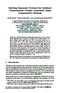
We suggest that the SRA-based method is as being sufficiently fast for practical applications in generation of simulation input data. In this report, we report properties of the successive random addition (SRA), one of recently proposed alternative methods for generating pseudo-random self-similar sequences. The C code of our implementation of the SRA algorithm is in Appendix A. This method can be characterised as follows by a diagram shown in Figure 1:

1 0

Interpolate midpoints

1

Add offsets to all points

Uniformly distributed Gaussian random random numbers numbers

Figure 1: SRA method

3

Normalisation

A self-similar sequence

The SRA method uses the midpoints like Random Midpoint Displacement (RMD) algorithm (for more detailed discussions, see [5]), but adds a displacement of a suitable variance to all of the points to increase stability of the generated sequence. The reason for interpolating midpoints is to construct Gaussian increments of X, which are correlated. Adding offsets to all points should make the resulted sequence self-similar and of normal distribution [20]. The SRA method consists of the following steps: Step.1 If the process {Xt } is to be computed for times instances t between 0 and 1, then start out by setting X0 = 0 and selecting X1 as a pseudo-random number from a Gaussian distribution with mean 0 and variance V ar[X1 ] = σ02 . Then V ar[X1 − X0 ] = σ02 . Step.2 Next, X 1 is constructed by the interpolation of the midpoint, that is, X 1 = 12 (X0 + X1 ). 2

2

S12

Step.3 Add a displacement of a variance (see the below how it is achieved.) to all of the points, i.e., X0 = X0 + d1,1 , X 1 = X 1 + d1,2 , X1 = X1 + d1,3 . The offsets d1,∗ are governed by fractional 2

2

Gaussian noise. For V ar[Xt2 − Xt1 ] = |t2 − t1 |2H σ02 to be true, for any t1 , t2 , 0 ≤ t1 ≤ t2 ≤ 1, it is required that V ar[X 1 − X0 ] = 14 V ar[X1 − X0 ] + 2S12 = ( 12 )2H σ02 , that is, S12 = 12 ( 211 )2H (1 − 22H−2 )σ02 .

2

Step.4 Next, Step.2 and Step.3 are repeated until the required numbers n of a sequence are reached. Therefore, Sn2 = 12 ( 21n )2H (1 − 22H−2 )σ02 , where σ02 is an initial variance and 0 < H < 1. Using the above steps, the SRA method generates an approximate self-similar FBM process.

4

Analysis of Self-Similar Sequences

The generator of self-similar sequences of pseudo-random numbers described in the Section 3 has been implemented in C on a Sun SPARCstation 4 (110 MHz, 32 MB), and used to generate selfsimilar cumulative arrival processes, mentioned at the end of Section 2. The mean times required for generating sequences of a given length were obtained by using the SunOS 5.5 date command and averaged over 30 iterations, having generated sequences of 32,768 (215 ), 131,072 (217 ), 262,144 (218 ), 524,288 (219 ) and 1,048,576 (220 ) numbers. We have also analysed the efficiency of the method in the sense of its accuracy. For each of H = 0.5, 0.55, 0.7, 0.9, 0.95, the method was used to generate over 100 sample sequences of 32,768 (215 ) numbers starting from different random seeds. Self-similarity and marginal distributions of the generated sequences were assessed by applying the best currently available techniques. These include: • Anderson-Darling goodness-of-fit test: used to show that the marginal distribution of sample sequences generated by the method is, as required, normal (or almost normal). This test is more powerful than Kolmogorov-Smirnov when testing against a specified normal distribution [7]. • Sequence plot: used to show that a generated sequence has LRD properties with the assumed H value. • Periodogram plot: used to show whether a generated sequence is LRD or not. It can be shown that if the autocorrelations were summable, then near the origin the periodogram should be scattered randomly around a constant. If the autocorrelations were non-summable, i.e., LRD, 4

Table 1: The numerical results of Anderson-Darling goodness-of-fit test

for normality at the 5% significance level are presented by percentages (%). For each of H = 0.5, 0.55, 0.7, 0.9, 0.95, the method was used to generate over 100 sample sequences of 32,768 (215 ) numbers starting from different random seeds. Each size of sample sequences is 32,768 numbers.

Method SRA

Theoretical Hurst parameter 0.5 0.55 0.7 0.9 0.95 97 97 95 58 32

the points of a sequence are scattered around a negative slope. The periodogram plot is obtained by plotting log10 (periodogram) against log10 (f requency). An estimate of the Hurst parameter ˆ = (1 − βˆ3 )/2 where βˆ3 is the slope [2]. is given by H • R/S statistic plot: graphical R/S analysis of empirical data can be used to estimate the Hurst parameter H. An estimate of H is given by the asymptotic slope βˆ2 of the R/S statistic plot, ˆ = βˆ2 [2]. i.e., H • Variance-time plot: is obtained by plotting log10 (V ar(X (m) )) against log10 (m) and by fitting a simple least square line through the resulting points in the plane. An estimate of the Hurst ˆ = 1 − βˆ1 /2 where βˆ1 is the slope [2]. parameter is given by H • Whittle’s approximate maximum likelihood estimate(MLE): is a more refined data analysis method to obtain confidence intervals (CIs) for the Hurst parameter H [2].

4.1

Analysis of Accuracy

We have summarised the results of our analysis in the following: • Anderson-Darling goodness-of-fit test was applied to test normality of sample sequences. The results of the tests, executed at the 5% significance level, showed that for H = 0.5, 0.55, 0.7, the generated sequences are normally distributed, but for H = 0.9, 0.95, they with the high value of H are weaker normally distributed than the former ones with the low value of H; see also Table 1. • Sequence plots in Figure 2 show higher levels of correlation of data as the H value increases. In other words, generated sequences have LRD properties. The estimates of Hurst parameter obtained from the periodogram, the R/S statistic, the variancetime and Whittle’s MLE, have been used to analyse the accuracy of the generator. The relative ˆ inaccuracy ∆H is calculated using the formula: ∆H = H−H H ∗ 100%, where H is the input value and ˆ H is an empirical mean value. The presented numerical results are all averaged over 100 sequences. • The periodogram plots have slopes decreasing as H increases and also see Figure 3. The negative slopes of all our plots for H = 0.5, 0.55, 0.7, 0.9, 0.95 were the evidence of self-similarity. The 5

Table 2: Relative inaccuracy ∆H estimated from periodogram plots.

Method SRA

.5 - 0.09 %

Theoretical Hurst parameter .55 .7 .9 - 1.41 % - 3.78 % - 5.13 %

.95 - 5.31 %

Table 3: Relative inaccuracy ∆H estimated from R/S statistic plots.

Method SRA

.5 +8.71 %

Theoretical Hurst parameter .55 .7 .9 +6.23 % +1.26 % - 4.44 %

.95 - 6.31 %

Table 4: Relative inaccuracy ∆H estimated from variance-time plots.

Method SRA

.5 - 2.76 %

Theoretical Hurst parameter .55 .7 .9 - 2.97 % - 3.38 % - 6.00 %

.95 - 7.47 %

relative inaccuracy ∆H of the estimated Hurst parameters of the method using periodogram plot is given in Table 2. We see that in the most cases parameter H of the SRA method was close to the required value, although the relative inaccuracy degrades with increasing H (but never exceeds 6%). The analysis of periodogram shows that the SRA method always produces ˆ self-similar sequences with negatively biased H. • The plots of R/S statistic clearly confirmed self-similar nature of the generated sequences and also see Figure 4. The relative inaccuracy ∆H of the estimated Hurst parameter, obtained by R/S statistic plot, is given in Table 3. The method of analysis of H does not link this generator ˆ as the periodogram plots did. with persistently negative or positive bias of H, • The variance-time plots also supported the claim that generated sequences were self-similar and also see Figure 5. Table 4 gives the relative inaccuracy ∆H of the estimated Hurst parameters obtained by the variance-time plot. Again, the method shows quality of the output sequences in the sense of H, with the relative inaccuracy increasing with the increase in H, but remaining ˆ below 8%. This time, the results suggest that the output sequences are negatively biased H. ˆ ± 1.96ˆ • The results for Whittle estimator of H with the corresponding 95% CIs H σHˆ , see Table 5, show that for all input H values, the SRA method produce sequences with negatively biased (except H = 0.5). Our results show that the generator produces approximately self-similar sequences, with the relative inaccuracy ∆H increasing with the increase of H, but always staying below 9%. Apparently there is a problem with more detailed studies of such a generator, since different methods of analysis of the ˆ characterising the same output Hurst parameter can give very different results regarding the bias of H 6

Table 5: Estimated mean values of H using Whittle’s MLE. Each CI is for over 100 sample sequences. 95% CIs for the means are given in parentheses.

Method SRA

.5 .500 (.490, .510)

Theoretical Hurst parameter .55 .7 .9 .538 .656 .825 (.528, .547) (.647, .666) (.816, .834)

.95 .869 (.860, .878)

Table 6: Complexity and mean running times of generators. Running times were obtained by using the SunOS 5.5 date command on a Sun SPARCstation 4 (110 MHz, 32 MB); each mean is averaged over 30 iterations.

Method

Complexity

SRA

O(n)

32,768 Numbers 0:3

Sequence of 131,072 262,144 524,288 1,048,576 Numbers Numbers Numbers Numbers Mean running time (minute:second) 0:10 0:20 0:40 1:31

sequences. More reliable methods for assessment of self-similarity in pseudo-random sequences are needed.

4.2

Computational Complexity

The results of our experimental analysis of mean times needed by the generator for generating pseudorandom self-similar sequences of a given length are shown in Table 6. The main conclusion is listed below. • The SRA method is fast. Table 6 shows its time complexity and the mean running time. It took 3 seconds to generate a sequence of 32,768 (215 ) numbers, while generation of a sequence with 1,048,576 (220 ) numbers took 1 minute and 31 seconds. The theoretical algorithmic complexity is O(n) [20]. In summary, our results show that a generator of pseudo-random self-similar sequences based on SRA is fast in practical applications, when long self-similar sequences of numbers are needed.

5

Conclusions

In this report we have presented the results of a generator, based on the SRA algorithm, of (long) pseudo-random self-similar sequences. It appears that this method generates approximately selfsimilar sequences, with the relative inaccuracy of the resulted H below 9%, if 0.5 ≤ H ≤ 0.95. On 7

the other hand, the analysis of mean times needed for generating sequences of given lengths shows that this generator should be recommended for practical simulation of computer networks, since it is very fast. Our study has also revealed that a more robust method for analysis of self-similarity in pseudo-random sequences is needed. This is the direction of our current research.

References [1] Beran, J. Statistical Methods for Data with Long Range Dependence. Statistical Science 7, 4 (1992), 404–427. [2] Beran, J. Statistics for Long-Memory Processes. Chapman and Hall, An International Thomson Publishing Company, 1994. [3] Cario, M., and Nelson, B. Numerical Methods for Fitting and Simulating Autoregressive-toAnything Processes. INFORMS Journal on Computing 10, 1 (1998), 72–81. [4] Cox, D. Long-Range Dependence: a Review. In Statistics: An Appraisal (1984), H. David and H. David, Eds., Iowa State Statistical Library, The Iowa State University Press, pp. 55–74. [5] Crilly, A., Earnshaw, R., and Jones, H. Fractals and Chaos. Springer-Verlag, 1991. [6] Garrett, M., and Willinger, W. Analysis, Modeling and Generation of Self-Similar VBR Video Traffic. In Computer Communication Review Proceedings of ACM SIGCOMM’94 (London, UK, Aug. 1994), vol. 24(4), pp. 269–280. [7] Gibbons, J., and Chakraborti, S. Nonparametric Statistical Inference. Marcel Dekker, Inc., 1992. [8] Granger, C. Long Memory Relationships and the Aggregation of Dynamic Models. Journal of Econometrics 14 (1980), 227–238. [9] Hosking, J. Modeling Persistence in Hydrological Time Series Using Fractional Differencing. Water Resources Research 20, 12 (Dec. 1984), 1898–1908. [10] Krunz, M., and Makowski, A. A Source Model for VBR Video Traffic Based on M/G/∞ Input Processes. In Proceedings of IEEE INFOCOM’98 (San Francisco, CA, USA, Mar. 1998), pp. 1441–1448. [11] Lau, W.-C., Erramilli, A., Wang, J., and Willinger, W. Self-Similar Traffic Generation: the Random Midpoint Displacement Algorithm and Its Properties. In Proceedings of IEEE ICC’95 (Seattle, WA, 1995), pp. 466–472. [12] Leland, W., Taqqu, M., Willinger, W., and Wilson, D. On the Self-Similar Nature of Ethernet Traffic(Extended Version). IEEE/ACM Transactions on Networking 2, 1 (Feb. 1994), 1–15. [13] Likhanov, N., Tsybakov, B., and Georganas, N. Analysis of an ATM Buffer with SelfSimilar(”Fractal”) Input Traffic. In Proceedings of IEEE INFOCOM’95 (1995), pp. 985–992. [14] Mandelbrot, B. A Fast Fractional Gaussian Noise Generator. Water Resources Research 7 (1971), 543–553. 8

[15] Mandelbrot, B., and Wallis, J. Computer Experiments with Fractional Gaussian Noises. Water Resources Research 5, 1 (1969), 228–267. [16] Neidhardt, A., and Wang, J. The Concept of Relevant Time Scales and Its Application to Queueing Analysis of Self-Similar Traffic (or Is Hurst Naughty or Nice?). In Proceedings ACM SIGMETRICS’98 (Madison, Wisconsin, USA, Jun. 1998), pp. 222–232. [17] Norros, I. A Storage Model with Self-Similar Input. Queueing Systems 16 (1994), 387–396. [18] Paxson, V. Fast Approximation of Self-Similar Network Traffic. Tech. Rep. LBL-36750, Lawrence Berkeley Laboratory and EECS Division,University of California, Berkeley, Apr. 1995. [19] Paxson, V., and Floyd, S. Wide-Area Traffic: the Failure of Poisson Modeling. IEEE/ACM Transactions on Networking 3, 3 (Jun. 1995), 226–244. [20] Peitgen, H.-O., and Saupe, D. The Science of Fractal Images. Springer-Verlag, 1988. [21] Rose, O. Traffic Modeling of Variable Bit Rate MPEG Video and Its Impacts on ATM Networks. PhD thesis, Bayerische Julus-Maximilians-Universitat Wurzburg, 1997. [22] Ryu, B. Fractal Network Traffic: from Understanding to Implications. PhD thesis, Graduate School of Arts and Science, Columbia University, 1996. [23] Taralp, T., Devetsikiotis, M., and Lambadaris, I. Efficient Fractional Gaussian Noise Generation Using the Spatial Renewal Process. In Proceedings IEEE International Communications Conference (ICC’98) (Atlanta, GA, USA, Jun. 1998), pp. S41–3.1–S41–3.5.

9

Appendix A

C Code for SRA Algorithm

/********************************************************** * SRA algorithm * * Description : * Saupe D. in Chapter 5 of "Fractals and Chaos" * edited by A.J. Crilly and R.A. Earnshaw and H. Jones, * Springer-Verlag, 1991. ********************************************************** * data: real array of size 2maxlevel + 1 * H: Hurst parameter (0 < H < 1) * maxlevel: maximum number of recursions * M: mean; V: variance **********************************************************/ void SRA-FBM(double *data, double H, int maxlevel, double M, double V) { /********************************************* * i,j,d,dhalf,n,level: integers * std: initial standard deviation * Delta[]: array holding standard deviations * gennor(M,V): normally distributed RNs using uniformly distributed RNs **********************************************/ int i,j,d,dhalf,n,level; double std; double Delta[maxlevel]; std=sqrt(1.0-pow(2.0,(2*H-2))); for(i=1; i