a generic enterprise resource ontology - Semantic Technologies Lab

Appeared in: Proceedings of the third IEEE Workshop on Enabling Technologies: Infrastructure for Collaborative Enterprises, April 1994, Morgantown, West Virginia (WET ICE ‘94)

A GENERIC ENTERPRISE RESOURCE ONTOLOGY Fadi George Fadel, Mark S. Fox, Michael Gruninger Department of Industrial Engineering, University of Toronto 4 Taddle Creek Road, Toronto, Ontario M5S 1A4 Canada tel:+1-416-978-6823 fax:+1-416-978-3453 internet: {fadel, msf, gruninger} @ie.utoronto.ca Abstract: The complexity of planning and scheduling is determined by the degree to which activities contend for resources. Accordingly this requires any application to have the ability to reason about the nature of the resource and its availability. This paper presents a generic enterprise resource ontology. The ontology described in this paper is one of many that is being created by the TOVE project in the Enterprise Integration Laboratory at the University of Toronto. Content Area: Enterprise Integration Frameworks

Modelling,

Enterprise

Keywords: Enterprise Modelling, Enterprise Ontology

1. Introduction The complexity of planning and scheduling is determined by the degree to which activities contend for resources. Accordingly this requires any application to have the ability to reason about the nature of the resource and its availability. This paper presents the ontology for modelling resources. Most information systems that support enterprise functions were created independently. This leads to three problems. Firstly, the functions do not share the same representations (i.e. different representations of the same enterprise knowledge); hence, they are unable to share knowledge. Secondly, the representations were defined without an adequate specification of what the terminology means (aka semantics); hence, the interpretations and uses of the knowledge are inconsistent. Thirdly, the representations lack any deductive capability; as a result, users are forced to spend significant effort on programming each new report or function that is required.

The key to integrating different enterprise functions, is to have the knowledge expressed with minimum assumptions of the application. The main aim of an ontology is to enable the coupling of enterprise functions and their respective knowledge and tools. In other words, the ontology acts as protocols for input, output and communication [Fox & Tenenbaum 90] [Gruber 91], creating efficient coordination and communication between different organizational units. Accordingly, the ontology provides a base representation for resources and a standard language of communication. The goal of the research is to create a Resource Ontology for a manufacturing enterprise. Manufacturing functions such as production planning and scheduling depend on the ability to reason about various facets of resources, such as their amounts, capacity and availability. In order to reason about these facets, a clear and precise representation must exist. The objectives of the research are: 1.

Define the span of the model by a set of competency questions.

2.

Create an ontology for resources.

3.

Implement the First Order Logic definition an constraints as axioms in Prolog.

The resource ontology described in this paper is one of many that is being created by the TOVE project in the Enterprise Integration Laboratory at the University of Toronto. The TOVE Project includes two major undertakings: the development of an Enterprise Ontology, and a testbed. The TOVE Enterprise Ontology provides a generic, reusable ontology for modelling enterprises. An ontology is comprised of a reference data model composed of objects, attributes and relations (also called the terms of

the ontology), and formal definitions of terms and their constraints in First Order Logic. The TOVE ontology currently spans knowledge of activity, state, time, causality, resources, cost and quality. The ontology’s data model is implemented on top of C++ using the Carnegie Group’s ROCKTM knowledge representation tool and the axioms are implemented in QuintusTM Prolog. The Prolog implementation provides a deductive mechanism (aka deductive database) which can be used to answer simple common sense questions without additional programming. The TOVE Testbed provides an environment for analyzing enterprise ontologies. The Testbed provides a model of an enterprise - a lamp manufacturing plant -, and tools for browsing, visualization, simulation and deductive queries.

2. Evaluation Criteria Though there exists a number of efforts seeking to create sharable representation of enterprise knowledge - CIMOSA [Esprit 90] , ICAM [Martin 83] , IWI [Scheer 89] , PERA [Williams 91] - little comparative analysis has been performed. Recently, two sets of evaluation criteria have been proposed. Fox & Tenenbaum have proposed the following criteria as a basis for evaluating an ontology: generality, efficiency, perspicuity, transformability, extensibility, granularity, scalability and competence [Fox & Tenenbaum 90] [Fox et al 93]. Gruber has proposed: clarity, coherence, extensibility, minimal encoding and minimal ontological commitment [Gruber 93]. The criterion we have chosen to evaluate our work is competence. The competence of a representation defines the types of tasks that the representation can be used in. Moreover, competency questions represent the starting point of the ontology development; the competency questions set the requirements for the ontology which in turn results in the modification of the competency questions. The obvious way to demonstrate competence is to define a set of questions that can be answered by the ontology. Given a representation and an accompanying theorem prover (such as Prolog), questions can be posed in the form of queries to be answered by the theorem prover. The creation of competency questions and an ontology is an iterative process; from the competency questions the ontology is derived which in turn results in a modification of the competency questions.

For example, in a study performed, over 30 managers from three different Westinghouse Corporation plants were asked to record the questions frequently asked [Fox 83]:

• What is the effect of the current state on the design and material specifications?

• What is the safe inventory level? • What is the effect of machine X breaking down on the product Z production?

• When is the expected finish time of the job j? • If order O is shipped then inform the client. • What are the required specifications that must be met by part X suppliers. These questions can serve as a set of competency questions for an enterprise model. Following are a subset of questions we have considered in the creation of the TOVE model.

• Divisibility: Can the resource be divided and still be usable?

• Quantity: What is the stock level at time t? • Location: Where is resource R? • Consumption: Is the resource consumed by the activity? If so, how much?

• Commitment: What activities is the resource committed to at time t?

• Structure: What are the subparts of resource R? • Capacity: Can the resource be shared with other activities?

• Trend: What is the capacity trend of a resource based on the machine usage history?

3. Resource Ontology We view that “being a resource” is not innate property of an object, but is a property that is derived from the role an object plays with respect to an activity. That is to say that properties of a resources determined by the activity. Accordingly, resources could be: Machines such as milling machines when associated with milling activities, Electricity or Raw materials consumed by an activity, Tools/Equipment such as fixtures, cranes, chairs etc., Capital needed to perform an activity, Human skill when needed to perform an activity, Information required to start an activity. In our analysis, we have strived to iden-

tify the primitive resource properties on which more complex properties, such as capacity recognition, are defined. Following are some examples of resource ontology* †.

• Resource-known: This is the most basic term in the ontology. It specifies knowledge of a resource as opposed to its physical existence. The importance of this definition lies in the fact that the ability to reason about a resource depends on it being known. rknown(R).

(PRO 1)

• Resource role: In TOVE, a resource has a role with respect to an activity. These roles are: raw material, product, facility, tool, operator. role(R, A, Role).

(PRO 2)

This entails that when a resource is defined as having a role with respect to an activity, then the resource can not have any other role with respect to the same activity. ∀(r, a, role1, role2) role(r, a, role1) ∧ role1 ≠ role2 ⊃ ¬ role(r, a, role2) (FOL 1)

A resource is physically divisible if the act of physically dividing the resource does not affect its role in the activity. In other words, the resource is physically divisible if each division can be used or consumed by the same activity‡. That property is useful for planner/ scheduler when deciding whether a portion of resource could support an activity. Functional divisibility of a resource, with respect to an activity, specifies that each division of the resource affects the functionality and not the structure of the resource. A parking lot is an example of such resources as the lot has a number of functional divisions that are used by parking activities. A “motor” is neither physically and functionally divisible when associated with “driving a car” activity. Finally, a resource is said to be temporal divisible if the use of a resource over time does not affect the future usability of the resource by the same activity. “A resource is physically divisible with respect to an activity if each physical division of the resource has the same role”. ∀(r, a) physical_divisible(r, a) ≡ ∀(r1, ro1) physical_division_of(r1, r) ∧ role(r1, a, ro1) ⊃ role(r, a, ro1)

• Division of: This term specifies that a resource could be divided. There are two types of divisions: physical, and functional. “Physical division of” specifies a division that is neither mental, moral or imaginary but is related to the division of the physical body of an object; “functional division of” specifies a division affecting the function and not structure. A “crank shaft” is a physical and a functional division of a “motor”. physical_division_of(R2, R).

(PRO 3)

functional_division_of(R2, R).

(PRO 4)

• Divisibility of a resource: This term specifies the property of a resource as being divisible with respect to an activity without affecting the role of the resource with respect to an activity. There are three types of divisibility: physical, functional and temporal divisibility.

*. For more examples and details please refer to [Fadel 94]. †. The first order logic formulation are tagged as (FOL #) while the Prolog implementation are tagged as (PRO #).

(FOL 2)

“A resource is functionally divisible with respect to an activity if each functional division of the resource has the same role”. ∀(r, a) functional_divisible(r, a) ≡ ∀(r1, ro1) functional_division_of(r1, r) ∧ role(r1, a, ro1) ⊃ role(r, a, ro1)

(FOL 3)

“A resource is temporally divisible with respect to an activity A1 if there exists a time period in which two activities, including A1, were executing with the condition that the first activity (A1) was either suspended or completed and the resource had the same role with both activities. Moreover, both activities were not executing simultaneously (i.e overlapping constraint).” ∀(r, a) temporal_divisible(r, a) ≡ ∃ (ti, ti1, ti2, tp1, tp2, a1, a2, s1, s2, role1) (uses(s1, r) ∨ consumes(s1, r)) ∧ (uses(s2, r) ∨ consumes(s2, r)) ∧ is_related(a1, s1)** ∧ is_related(a2, s2) ∧ time_bound(s1, ti1)†† ∧ time_bound(s2, ti2) ∧ ‡. i.e each division shares the same role of the original resource. **. is a term defined in the activity-state ontology specifies an activity is linked (related) to a state.

activity(a1,executing,tp1)*∧period_contains(ti1, tp1)† ∧ ((activity(a1,suspended,tp_end)∧tp_end =EP(ti1)‡) ∨ ((activity(a1, completed,tp_end) ∧ tp_end = EP(ti1)) ∧ activity(a2, executing, tp2) ∧ period_contains(ti2, tp2) ∧ ¬overlaps(ti1,ti2) ∧contains(ti, ti1) ∧contains(ti, ti2) ∧ role(r, a1, role1) ∧ role(r, a2, role1)

• Component of: “Component of” specifies a resource as being a part of another resource implying that a resource consists of one or more sub-resources (i.e sub components). A resource can be a physical or functional component of another resource with respect to an activity and each does not share the same role with the original resource. This term is used for example in the bills of material explosion of parts. “A resource R2 is a physical component of resource R1 if R2 is a physical division of the R1 and both resources do not share the same role with respect to an activity”. ∀(r1, r2) physical_component_of(r2, r1) ≡ ∀(a, r, ro1) physical_division_of(r2, r1) ∧

(FOL 4)

• Unit of measurement: This predicate specifies a default measurement unit for a resource, when associated with activity. Accordingly, resource quantity or capacity is to be measured using the specified unit of measurement. This term is used for specifying both the qualitative and quantitative units of measurement. Qualitative units of measurement consist of an ordered set such as {large, medium small}. Qualitative units can be also used as a measure of quality: {good, bad}. Quantitative units are used to specify attributes such as weight, length, capacity. unit_of_measurement(R,Unit_ID,Unit,A).(PRO 5)

role(r2, a, ro1) ⊃ ¬role(r1, a, ro1)

(FOL 6)

“A resource R2 is a functional component of resource R1 if R2 is a functional division of the R1 and both resources do not share the same role with respect to an activity”. ∀(r1, r2) functional_component_of(r2, r1) ≡ ∀(a, r, ro1) functional_division_of(r2, r1) ∧ role(r2, a, ro1) ⊃ ¬role(r1, a, ro1)

(FOL 7)

• Quantity: A resource point (rp) specifies a resource’s quantity at a some time and unit of measure.

• Measured by: “Measured by” defines the objects by which a resource is measured with respect to an activity. This term acts as a constraint on the “unit of measurement” term. Each unit of measure must have a corresponding “measured by” assertion. measured_by(R, Unit_id, A).

(PRO 6)

As mentioned, a constraint on the “unit of measurement” is that there should be a corresponding measured by assertion (∀ r) (∃ unit_id, a) measured_by(r, unit_id, a) ⊃ (∃ u) unit_of_measurement(r, unit_id, u, a) (FOL 5)

††. time_bound(s,ti) specifies that ti is the time of interval of the state. *. activity(a1, executing, tp1) specifies that activity a1 has to be executing at time point tp1. †. period_contains(ti, tp) specifies that time point tp is contained by ti time period. ‡. EP(ti) is function that returns the end time point of an interval.

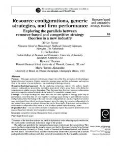
figure 1 3-D resource point - in terms of quantity, time and location rp(Unit) 5 4 3 2 1

L1

L1

L1

1

2

3

L1

L2 4

L3

L1

L2

L3

5 time horizon

figure 2 2-D resource point - in terms of quantity and time rp(unit) 5 4 3 2 1 1 2 3 4 5 6 7 8 9 time horizon

We have defined two resource point terms - 3-D and 2-D definitions. The 3-D definition (figure 1) is asserted as a ground term and is defined in terms of time, location and quantity* while the 2-D definition (figure 2) represents resource amounts aggregated across all locations and is calculated using 3-D rp assertions†. rpl(plug, 100, tp90, ss12, unit).(PRO 7)

For example the above assertion, 3-D rpl definition, specifies the existence of a resource point for resource plug at time point tp90, with quantity of 100 units at location ss12. ?- rp(resource, Q, time, unit). (PRO 8)

The 2-D resource point definition returns the summation of all resource point quantities for resource, over all locations at a specific time point. Besides that ability to represent physical resource quantities, resource point is also used for the identification of capacity of reusable resources such as in the example of ftp site where rp would denote to the unused accessed lines.

• Application specification: The predicates in this section are defined for notational convenience. The consumption, use and produce specifications specify the amounts of the resource that is to be consumed, used or produced respectively over a time interval as well as the unit of measurement. The information included in these specifications‡ are already defined in the activity state ontology. There are three application specification: consumption, use and production specifications. consumption_spec(R,A,Ti,Q,Rate, Unit).(PRO 9) use_spec(R,A,Ti,Q,Rate,Unit).

(PRO 10)

produce_spec(R,A,Q,Rate,Ti,Unit). (PRO 11)

where Q represent the total number consumed/produced by an activity or the portion of the resource used by an activity. The application specification, consumption specification for example, concatenates the specification into one term as defined in the following FOL formulation: *. rpl(resource, quantity, time_point, locations, unit). †. rp(resource, quantity, time_point, unit). ‡. i.e the arguments of each term

(∃ a, q, ti, u) (∀r) consumption_spec(r, a, q, ti, u) ≡ (∃ s, s2, unit_id) enabling(s, a) ∧ is_related(a,s2,) ∧ consumes(s2, r)** ∧ quantity(s2, q)†† ∧ time_bound(s2, ti)‡‡ ∧ unit_of_measurement(r, unit_id, u, a) ∧ measured_by(r, unit_id, a)

(FOL 8)

“The consumption specification term entails that the resource amount will be decremented after the completion of the activity”*** †††. (∀r, a, s, ti, q’, rate, unit) consumption_spec(r, a, ti, q’, rate, unit) ≡ (∀ s, r, a, q, ti, tp, tp’) rp(r, q, tp, unit_id) ∧ ((is_related(a, s) ∧ consumes(s, r)) ∧tp = SP(ti) ∧ tp’ = EP(ti)∧ enabling_state(s, tp, enabled) ⊃ rp(r, q - q’, tp', unit)

(FOL 9)

“The use specification term entails that the resource amount will remain constant, if the resource is being used” (∀r, a, s, ti, q’, rate, unit) use_spec(r, a, s, ti, q’, rate, unit) ≡ (∀ s, r, a, q, ti, tp, tp’) rp(r, q, tp, unit_id) ∧ (is_related(a, s) ∧ uses(s, r)) ∧tp = SP(ti) ∧ tp’ = EP(ti) ∧ enabling_state(s, tp, enabled) ⊃ rp(r, q, tp', unit)

(FOL 10)

“The produce specification term entails that the resource amount will increase by a constant, if the resource is being used”. (∀r, a, s, ti, q’, rate, unit) produce_spec(r, a, s, ti, q’, rate, unit) ≡ (∀ s,r,a,q,ti,tp,tp’) rp(r, q, tp, unit_id) ∧ (is_related(a, s) ∧ produces(s, r)) ∧ tp = SP(ti) ∧ tp’ = EP(ti) ∧ enabling_state(s, tp, enabled) ⊃ rp(r, q + q’, tp', unit)

(FOL 11)

**. consumes(s2,r) specifies that state s2 consumes resource r. ††. quantity(s2, q) specifies that state s2 requires q of the resource. ‡‡. time_bound(s2, ti) specifies that ti is the time interval of s2 state ***. Reiter discusses effect axioms in [Reiter 91]. In TOVE, there are number of effect axioms and the committed-related ones are some examples [TOVE 92] [Gruninger & Fox 94]. †††. SP(ti) represents that starting point of time period ti, while EP(ti) represents the end point of time interval ti.

• Continuous vs. discrete resources: A continuous

• Simultaneous Use Restriction: Simultaneous use

resource indicates a resource that is uncountable. These resources are marked by uninterrupted extension in volume. Discrete resources on the other hand specify that a resource is countable. These terms are defined relative to an activity.

restriction prohibits the use/consumption of a resource by two activities simultaneously. For example, this term is used to specify that two activities can not use the resource “oven” simultaneously as both activities require different operating temperature†.

(∀ r, a) [continuous(r, a) ≡ physical_divisible(r, a)] (FOL 12)

The predicate is defined as ground term with the following parameters:

(∀ r, a) [discrete(r, a) ≡ ¬ continuous(r, a)]

(FOL 13)

The implication of the above is if the resource is discrete and the consumption or the use specification is defined in terms of integer amounts*. ∀(r, a, q, ti, u) (consumption_spec(r, a, q, rate,ti, u) ∨ use_spec(r, a, q, rate,ti, u)) ∧ discrete(r, a) ⊃ integer(q)

(FOL 14)

• Usage Mode: Usage mode axiom returns whether a resource supports an activity on a discrete or continuous basis. The term does not imply that the activity is discrete or continuous. The mode of usage is depended on the activity that uses/consumes the resource. “The mode of usage is achieved through checking the use/consume/produce specification term. If the of the quantity term (Q) is equal to the rate term (Rate) in the specification, then the process is discrete otherwise the process is continuous with a rate which is equal to the rate parameter” (∀ r, a) continuous_mode(r, a) ≡ (∃ q, unit, rate, ti) ((use_spec(r, a, ti, q, rate, unit) ∨ consumption_spec(r, a, ti, q, rate, unit) ∨ produce_spec(r, a, ti, q, rate, unit)) ∧q ≠ rate (FOL 15) (∀ r, a) discrete_mode(r, a) ≡ (∃ q, u, rate, unit) ((use_spec(r, a, ti, q, q, unit) ∨ consumption_spec(r, a, ti, q, q, unit) ∨ produce_spec(r, a, ti, q, q, unit))

(FOL 16)

If a usage mode of a resource is continuous with respect to an activity, that implies that the resource is continuous.

• A1: activity ID of the first activity using a resource.

• A2: activity ID of the second activity using a resource.

• R: ID of the resource to be used. simultaneous_use_restriction(A1, A2, R).(PRO 12)

This term specifies that activities A1 and A2 can not be supported by resource R at the same time. This entails that both activities can not commit the resource over two overlapping intervals. (∀ a1, a2, r) simultaneous_use_restriction(a1, a2, r) ≡ (∀ s, s2, r, a, a2) (¬ ∃t) use(s, a) ∧ uses(s, r) ∧ use(s2, a2) ∧ uses(s2, r) ⊃ enabling_state(s, tp, enabled) ∧ enabling_state(s2, tp, enabled)

(FOL 18)

• Committed to: This predicate to specifies the commitment of a resource to an activity thereby making the resource partly/fully unusable/inconsumable by any other activity. A resource is committed to an activity as a result of a scheduling activity. Committed_to is defined as a ground term with the following parameters:

• R: ID of the resource to be used/consumed. • A: ID of the activity to use/consume the resource.

• S: the ID of the state that is satisfied by the assertion of the committed term.

• Ti: the ID of the time interval of the activity. • Amount: amount of the resource that is committed to an activity.

(∀r,a)continuous_mode(r,a)≡continuous(r,a)(FOL 17)

*. integer(q) is used specifying that q is an integer

†. this term is also use case one activity negatively interacts with the other

• Unit: unit of measurement. committed_to(R, A, S, Ti,Amount, Unit).(PRO 13)

“A constraint on the committed to term is that the time interval of commitment should either be equal or greater than that is defined in the specification”. (∀r, a, s, ti, ti2, q, q’, rate, unit) committed_to(r,a,s,ti,q’,u) ∧ (consumption_spec(r, a, ti2, q, rate, unit) ∨ use_spec(r, a, ti2, q, rate, unit)) ⊃ (contains(ti, ti2) ∨ equal(ti, ti2))

(FOL 19)

• Total Committed: This predicate specifies the total amount committed of a resource to all activities at a specified time point. The total commitment of a resource is defined to be the summation of all amount committed of resources to all activities. The first order logic would be in the form of: (∀ r, tp, u) (∃ TQ) total_committed(r, TQ, tp, u) ≡ (∃ pd1, pd2 … pdn, a1, a2 … an, q1, q2 … qn) committed_to(r,a1,pd1,q1,u) ∧ period_contains(ti, pd1) ∧ (committed_to(r, a2, pd2, q2, u) ∧ …… ∧ c ommitted_to(r, an, pd2, qn, u) ∧ TQ = q1+ q2 + …+ qn

(FOL 20)

“An effect of a resource being committed is that after the completion of the activity the total amount committed will be decremented”*. (∀ s, r, a, q, q’, ti, tp, tp’, u) ((use(s, a) ∧ uses(s, r)) ∨ (consume(s, a) ∧ consumes(s, r)))∧ total_committed(r, q’, tp, u) ∧ enabling_state(s, tp, possible) ∧ (tp = SP(ti)) ∧ (tp’ = EP(ti)) ⊃ total_committed(r, q - q’, tp’, u)

(FOL 21)

• Capacity: Capacity is defined to be the maximum set of activities that can simultaneously use/consume a resource at a specific time. In the case where the resource is physically indivisible then the capacity denotes an activity that could use/consume the resource. On the other hand if the resource is physi-

*. In TOVE, this axiom is called an effect axioms which links the resource ontology with the causal theory of activity [Fadel et al 94].

cally divisible†, capacity represents the number of activities that a resource can support simultaneously. The complexity of the process of determining the capacity of a resource depends on the activities requiring the resource and the activities already supported by the resource. Capacity determination problem is reducible to the scheduling problem. The capacity recognition process is solvable in polynomial time in the case where the activities using/consuming the resource are homogenous. Homogeneity implies that activities require equivalent amounts of the resource and processing time or integral multiple thereof. Accordingly the output of the capacity recognition process is reducible to a number which represents the number of activities that the resource could be allocated to. The process becomes complex in the case where the activities requiring the resource are heterogenous. Finding the maximum set of activities is reducible to a single machine scheduling problem which is NP-hard. If the resource is functionally divisible, then the process becomes NP-hard in the strongest sense as the resource can support multiple activities simultaneously. What is required is a sequencing heuristic for a number of activities that are to use or consume a resource in a predetermined time window. The sequencing heuristic is to be defined for a certain objective such as to minimize the number of tardy activities. One of the terms defined for the capacity recognition process is available for. A resource is available for an activity if the resource’s quantity can support the activity and there is no simultaneous use restriction between the activity requiring the resource and the ones already supported by the resource. Following is a logical specification of this definition: (∀r) (∃a, ti,) available_for(r, [a], ti) ≡ (∀ tp ∈ ti) (∃ unit_id, u, amt_required, tq, q, amount1, amount2 … amountn, rate1, rate2 … raten) (consumption_spec(r, a1, ti, amount1, rate1, unit) ∨ use_spec(r, a1, ti, amount1, rate1, unit)) ∧ (consumption_spec(r, a2, ti, amount2, rate2, unit) ∨ use_spec(r, a2, ti, amount2, rate2, unit)) ∧ …… ∧ (consumption_spec(r, an, ti, amountn, raten, unit) ∨ use_spec(r, a, ti, amountn, raten, unit)) ∧ amt_required = amount1+amount2 + ……+amountn ∧ (period_contains(ti, tp) ∧

†. implying having the ability being shared by multiple activities.

(total_committed(r, tq, tp, unit))∧ unit_of_measurement(r, unit_id, u, a) ∧ measured_by(r, unit_id, a) ∧ rp(r, q, tp, unit) ∧ (amt_required ≥ q- tq) ∧ ((∀ax ∈ a) no_restricition(r, a, ax, ti))

(FOL 22)

resource_configuration(r, c1, a1) ∧ ¬resource_configuration(r, c1, a2) ⊃ simultaneous_use_restriction(a1, r, a2)

no_restricition(r,a,ax,ti) ≡ (committed_to(r,ax,s,ti2,q,u) ∧ (a ≠ ax) ∧ period_overlaps(ti, ti2) ∧ ¬(simultaneous_use_restriction(a, ax, r)))

(FOL 23)

• Activity history: This predicate specifies the history of usage or consumption of a resource before a specified time point. A list of activities that were supported by the resource will be returned. “An activity will be included in the list of activities, that were supported by the resource, if the resource was committed to the activity for a time period with end time less or equal than the specified time point”. (∀ r) (∃act_list, tp) activity_history(r, act_list, tp) ≡ (∀ a∈ act_list)(∃ti, q, u, a, s) (committed_to(r, a, s, ti, q, u) ∧ period_before(ti, tp) ∧ enabling_state(s, tp, completed)

(∀ a1, a2, r) (∃ q1, q2, ti1, ti2, rate1, rate2, c1) (use_spec(r, a1, ti1, q1, rate1, u) ∨ consumption_spec(r, a1, ti1, q1, rate1, u))∧ (use_spec(r, a2, ti2, q1, rate2, u) ∨ consumption_spec(r, a2, ti2, q1, rate2, u)) ∧

(FOL 24)

• Resource configuration: This term specifies the configuration of a resource with respect to an activity. This term implies that for the activity to the resource must have the specified configuration. Moreover, after the completion of the activity, C is going to be the configuration of the resource unless changed. This term is divided as a ground term with three arguments:

• R: resource ID • C: ID specifying the configuration of the resource

• A: activity with which the resource has C configuration resource_configuration(R, C, A). (PRO 14)

This implies that if activities a1 and a2 require the same resource but both activities require different configuration, then that implies that the resource can not support both activities simultaneously (i.e there is a simultaneous use restriction constraint).

(FOL 25)

• Set up constraint: Set-up term specifies the duration required to set-up a resource for usage by an activity. The set time is defined with regards to pair of activities. The set-up time includes configuration and location dependent time. In the configuration set-up time, the specified duration as a function of the time required to change the resource’s configuration state, as result of the last activity supported, to that implied by the activity requiring the resource. As for the location set-up time, it specifies the duration required for the resource to transport or be transported from one location to another. “Set up time is equal to the time required to change the resource’s configuration. If the resource needs to relocated, then the set up time also includes the time of transportation” (∀ r, a2, l2, dur, u) set_up(r, a2, l2, dur, u) ≡ (∃ a1, ti, q, c, tp1, l1, ct, lt, u2, s1) committed_to(r, a1, s1, ti, q, u) ∧ tp = EP(ti) ∧ resource_configuration(r, c, a) ∧ rpl(r, q, tp1, l1, u) ∧ (config_set_up(r, a1, a2, ct, u2) ∧ loc_set_up(r, l1, l2, lt, u2) ∧ dur = ct + lt)

(FOL 26)

The set-up duration is the summation of the configuration and location dependent set-up times. If the resource is not to be moved from a location*, then the set up time id only the time needed to re-configure the resource. Configuration set-up time (config_set_up) is defined as a ground term with these arguments:

• R: resource ID • A1: the activity that caused the last configuration change of the resource

*. i.e already in the location required by the activity

• A2: activity requiring the change in the configuration of the resource

• CT: configuration dependent set-up time • Unit: temporal unit of measurement config_set_up(R, A1, A2, CT, Unit).

(PRO 15)

Location set-up time is defined as a ground term with five arguments:

• R: resource ID • L1: the location from which the resource is to be relocated

• L2: destination of the resource • LT: location dependent set-up time • Unit: temporal unit of measurement loc_set_up(R, L1, L2, LT, Unit). (PRO 16)

• Alternative resource: This term specifies an alternative resource(s) to be used or consumed by an activity. This is useful in the case when an alternative resource is required because of a machine breakdown or unavailability of a resource. “There exist an alternative resource for an activity, if there exists a disjunct non-terminal enabling state” (∀ r, a) (∃ list) alternative_resource(r, a, list) ≡ (∃ s, s2, disjunct_state) uses(s2, r) ∧ is_related(s2, s) ∧ subclass_of(s, disjunct_state)

(FOL 27)

• Relation between resource ontology and activitystate ontology: A state in TOVE represents what has to be true in the world in order for an activity to be performed, or what is true in the world after the completion of an activity. The status of a state, and any activity, is dependent on the status of resources that the activity uses or consumes. One of the status that a state could have is possible. A consume state* could be possible if:

• the resource is available for the activity and • the resource has not been committed yet to the resource and

• the activity is not executing. *. i.e the state of an activity consuming a resource.

(∀ state_id) (∃ tp) possible(state_id, tp) ≡ (∃ r, a, ti, unit) (consume(state_id, a) ∨ consumes(state_id, r)) ∨ (use(state_id, a) ∨ uses(state_id, r)) ∧ available_for(r, a, ti) ∧ ¬committed_to(r, a, state_id, ti, amount, unit) ∧ period_contains(ti, tp) ∧ ¬activity(a, executing, tp)†

(FOL 28)

Moreover a consume state is completed if:

• the activity is in the activity history of the resource. (∀ state_id) (∃ tp) completed(state_id, tp) ≡ (∃ r, a, act_list) ((consume(state_id, a) ∧ consumes(state_id, r)) ∨ (use(state_id, a) ∧ uses(state_id, r))) ∧ activity_history(r, act_list, tp) ∧ member_of(a, act_list) (FOL 29)

4. Examples of competency questions: Recall that the competency questions are the basis (starting point) of ontology development. Similar to the approach in defining the ontology, competency questions are defined starting with the most simple questions‡. What is presented in this section is some examples of competency questions and their Prolog implementation**; it shows how the ability to answer a query depends on the availability of number of ontologies. ☞ ☞ Is there enough capacity for the performance of “fabricate_short_shaft_1” and “fabricate_short_shaft_2” activities on the “mold1” resource in the next hour? (Given a number of activities requiring the resource mold1, what is the capacity of the resource during a time period?) |?- available_for(mold1, [fabricate_short_shaft_1, fabricate_short_shaft_2], pd3, Result)††.

†. activity(a, executing, tp) specifies that activity a is executing at time point tp. ‡. i.e the competency are stratified. **. A query in Prolog is proceeded by “|?-”. A variable is represented as capital letters. ††. Figures 3 and 4 present a taxonomy of ontology and axioms required to answer the query.

figure 3 ”available for” requires the following ontology Requires |?- functional_division_of(R, mold1). no. division_of is usedto reason about the sharability of the resource resource.(i.e used indivisible term) |?- physical_division_of(R2, mold1). R2 = rectangle_1; no |?-unit_of_measurement(mold1,Unit_ID, U, fabricate_short_shaft_1). Unit_ID = rectangle_1 U = rectangle_1; no |?- functional_divisible(mold1, fabricate_short_shaft_1). yes |?- use_specification(mold1, fabricate_short_shaft_1,pd1,30,30, recatngle_1). Q = 30; no |?- total_committed(mold1, TQ, tp, rectangle_1). TQ = 30; no |?- rpl(mold1, Q, tp2, rectangle_1). Q = 150; no

figure 4 ”available for” requires the following ontology -cont’d continuation of last figure |?- has_current_activity(mold1,List, tp). . . has_current_activity is used to . to find out if the activities . requiring and supported by the resource are homogenous/ . heterogenous . . Requires . . |?-committed_to(mold1,A,S,_,tp, rectangle_1). . A = fabricate_short_shaft_2 . S = es_fabricate_short_shaft_2; . no . . |?-enabling_state( . fabricate_short_shaft_2,tp, Status). . Status = enabled; . no .

List = assemble_clip_reading_lamp, assemble_hand; no temporal ontology (e.g before, after) Result = [fabricate_short_shaft_1]; no

|?- simultaneous_use_restriction( fabricate_shirt_shaft_1, A2, mold1). no. simultaneous_use_restriction is used so that no two confliction activities can use resource simultaneously

continued next figure

the resource has the capacity to only support fabricate_short_shaft_1 activity A smooth production requires the availability of resources at the time of productions. Resources should be replenished before the stock reaches a certain limit and that is checked through using the following query. ☞ ☞ Is the stock for short_shaft in danger of being depleted between now and the end of the week?* |?- rp(short_shaft, Q, Tp), Tp > now, Tp < tp333, Q < 20.

*. i.e will the resource point fall below then a certain value

Q = 15 Tp = tp23;

figure 6 “physical component of” requires Requires

Q = 10

|?- physical_division_of(R2, clip_reading_lamp).

Tp = tp200;

|?- role(R2, fabricate_short_shaft_1, tool).

no

Assignment of resources (or alternative resources) is a crucial function in a manufacturing environment. This is used in case of resource unavailability, for example, due to a machine breakdown or delay in a shipment.

each physical division should not share the same role with the original resource

☞ ☞ Can resource mold2 be used instead of resource mold1? (Is mold2 an alternative resource of mold1 for activity fabricate_short_shaft?)

R = clip_base

|?- alternative_resource(mold1, fabricate_short_shaft, List), member_of(mold2, List).

R = short_arm

figure 5 “alternative resource” requires Requires activity state ontology. |?- role(R2, fabricate_short_shaft_1, tool). yes the alternative resources has to have same role

List = [mold2]; no mold2 is an alternative resource for the activity fabricate_short_shaft_1

Another important function in planning is to be able to explode the bill of material of a resource. ☞ ☞ What are the components of resource clip_reading_lamp? (What are the physical component of the resource?) |?- physical_component_of(R, clip_reading_lamp, A, Type).

A = assemble_clip_reading_lamp Type = physical;

A = assemble_clip_reading_lamp Type = physical; R = small_head A = assemble_clip_reading_lamp Type = physical; no

5. Conclusion In this paper we have presented an ontology for resources in a manufacturing enterprise environment. This ontology has the characteristics of being generic and reusable over a wide variety of applications. The ontology provides the capability of deductively answering common sense questions about the enterprise knowledge. In particular it us to reason about how properties of resources change as the result of activities, and also to reason about the allocation of resources in a scheduling task through capacity recognition. This work lays the foundation for further research in additional planning, scheduling and modelling tasks in enterprise engineering.

6. Acknowledgments This research is supported, in part, by the Natural Science and Engineering Research Council, Carnegie Group Inc., Quintus Corp., Digital Equipment Corp., Micro Electronics and Computer Research Corp., and Spar Aerospace.

7. References [Esprit 90]ESPRIT-AMICE. CIM-OSA - A Vendor Independent CIM Architecture. Proceedings of CINCOM 90, pages 177-196. National Institute for Standards and Technology, 1990.

[Reiter 91]Reiter, R., The frame problem in the situation calculus: A simple solution (sometimes) and a completeness result for goal regression. Artificial Intelligence and Mathematical Theory of Computation: Papers in Honor of John McCarthy. Academic Press, San Diego, 1991.

[Fadel 94]Fadel, Fadi George, Microtheory of resources, M.A.Sc thesis, University of Toronto, to be published 1994.

[Scheer 89]Scheer, A-W. Enterprise-Wide Data Modelling: Information Systems in Industry. Springer-Verlag, 1989.

[Fox 83] Fox, M.S.,The Intelligent Management System: An Overview, Processes and Tools for Decision Support, North-Holland Publishing Company, 1983.

[TOVE 92]Fox, Mark S., Chionglo, John, Fadel, Fadi George, The TOronto Virtual Enterprise model, Enterprise Integration Laboratory, University of Toronto, 1993.

[Fox & Tenenbaum 90] Fox, M.S., and Tenenbaum, J.M., (1991), Proceedings of the DARPA Knowledge Sharing Workshop, Santa Barbara Ca.

[Williams 91]Williams, T.J., and the Members, IndustryPurdue University Consortium for CIM. The PURDUE Enterprise Reference Architecture. Technical Report Number 154, Purdue Laboratory for Applied Industrial Control, Purdue University, West Lafayette, IN 47907, 1991.

[Fox et al 93]Fox, Mark S., Chionglo, John F., Fadel, Fadi G., Towards Common Sense Modelling of an Enterprise, Proceeding of the Second Industrial Engineering Research Conference, 1993. [Fox & Gruninger 94] Fox, Mark S., Gruninger, Michael, Ontology for activity for Enterprise Engineering, submitted to Twelfth National Conference on Artificial Intelligence (AAAI-94). [Gruber 91]Gruber, Thomas R., The Role of Standard Knowledge Representation for Sharing Knowledge-Based Technology, To appear in: Allen, J. A., Fikes, R., and Sandewell, E. (Eds) Principles of Knowledge Representation and Reasoning: Proceedings of the Second International Conference, 1991. [Gruber 93]Gruber, Thomas R., Toward Principles for the Design of Ontologies Used for Knowledge Sharing, KSL 93-4, Computer Science Department, Stanford University, 1993. [Martin 83]Martin, C., and Smith, S. Integrated Computeraided Manufacturing (ICAM) Architecture Part III/Volume IV: Composite Information Model of “Design Product” (DES1). Technical Report AFWAL-TR-82-4063 Volume IV, Materials Laboratory, Air Force Wright Aeronautical Laboratories, Air Force Systems Command, Wright-Patterson Air Force Base, Ohio 45433, 1983.