A Generic Scheme for Combining Multiple ... - Semantic Scholar

A Generic Scheme for Combining Multiple Inclusion Representations in Numerical Constraint Propagation Xuan-Ha Vu, Djamila Sam-Haroud, and Boi V. Faltings Artificial Intelligence Laboratory, Swiss Federal Institute of Technology in Lausanne (EPFL), CH-1015, Lausanne, Switzerland {xuan-ha.vu, jamila.sam, boi.faltings}@epfl.ch http://liawww.epfl.ch Technical Report No. IC/2004/39 (April 21, 2004)

Abstract. This paper proposes a novel generic scheme enabling the combination of multiple inclusion representations to propagate numerical constraints. The scheme allows bringing into the constraint propagation framework the strength of inclusion techniques coming from different areas such as interval arithmetic, affine arithmetic or mathematical programming. The scheme is based on the DAG representation of the constraint system. This enables devising fine-grained combination strategies involving any factorable constraint system. The paper presents several possible combination strategies for creating practical instances of the generic scheme. The experiments reported on a particular instance using interval propagation, interval arithmetic, affine arithmetic and linear programming illustrate the flexibility and efficiency of the approach.

1

Introduction

Many real world applications involve the solving of problems modeled as numerical constraints on variables with continuous domains. In practice, numerical constraints can be equalities or inequalities of arbitrary type, usually expressed in factorable form, that is, they can be represented by elementary functions such as +, −, ×, ÷, log, exp, sin, cos, . . . Recently, many solution techniques have been proposed in constraint programming to solve such constraint systems. Some of them are based on interval (constraint) propagation and interval arithmetic (e.g. the works in [1], [2] and references therein), while some of them are based on linear relaxation and linear programming ([3], [4]). There have also been techniques ([5], [6]) that use G interval or affine arithmetic to solve equation systems. Most of the solution techniques are interleaved with a bisection search (or similar) to solve the problems exhaustively. Lately, there have been some advanced search techniques ([7], [8]) that improve the search performance for problems with nonisolated solutions (e.g., inequalities) while maintaining the same performance

2

X.-H. Vu, D. Sam-Haroud and B. Faltings

for problems with isolated solutions (e.g., equalities). In general, different techniques have different strengths that are complementary. Therefore, combining the strength of different solution techniques is the subject of intensive research efforts (see [2] and references therein). Our contributions will be described in Section 3 and Section 4. In Section 3, we propose a novel generic scheme which allows devising new combination strategies for numerical constraint propagation in a flexible way. The scheme enables the propagation to be performed using different inclusion representations on a directed acyclic graph (DAG) that represents the problem. Consequently, the scheme is applicable to any factorable constraint system. The goal is to provide a combination scheme that is efficient and flexible but still general enough to bring the strength of different solution techniques coming from different areas (e.g., constraint programming and mathematical programming) into the framework of constraint propagation. In order to illustrate the flexibility and efficiency of the proposed scheme, in Section 4 we propose improvements on affine arithmetic and then devise from the scheme several new combination strategies which are based on emerging techniques, namely interval constraint propagation, interval arithmetic, affine arithmetic, and linear programming. In Section 5, our experiments show that the devised technique is superior than the recent interval propagation methods in performance and quality. It even outperforms some very recent techniques in mathematical programming and constraint programming which are specially designed to solve certain constraint systems. The conclusion and future directions are given in Section 6.

2 2.1

Background and Definitions Interval Arithmetic

When using an interval [a, b] ⊆ R to represent a quantity x, we mean that for each value assigned to x, the following holds a≤x≤b

(1)

There have been different variants of the interval notion that are still valid for the techniques proposed in this paper, however, for simplicity we use the term “interval” to refer to the notion defined by (1). Interval arithmetic is an arithmetic defined on the set of intervals, rather than the set of real numbers. According to a survey paper [9], a form of interval arithmetic perhaps first appeared in 1924 in [10], then later in [11]. Modern development of interval arithmetic began with R. E. Moore’s dissertation [12] and R. E. Moore’s book [13]. Another good introduction to interval arithmetic can be found in [14]. Interval arithmetic has been being used to solve numerical problems with guaranteed accuracy. Fundamentally, if x and y are two real intervals, then the four elementary operations for idealized interval arithmetic obey the rule x ¦ y = {x ¦ y | x ∈ x, y ∈ y}, ∀¦ ∈ {+, −, ×, ÷}

(2)

A Combination Scheme for Numerical Constraint Propagation

3

Thus, the ranges of the four elementary interval arithmetic operations are exactly the ranges of the their real-valued counterparts. Although the rule (2) characterizes these operations mathematically, interval arithmetic’s usefulness is due to the operational definitions based on interval bounds [15]. For example, if x = [x, x] and y = [y, y], we then have: x + y = [x + y, x + y] x − y = [x − y, x − y] x × y = [min{xy, xy, xy, xy}, max{xy, xy, xy, xy}] 1/x = [1/x, 1/x], if x > 0 or x < 0 x ÷ y = x × 1/y Moreover, if such operations are composed, bounds on the ranges of real functions can be obtained. For example, if given the function f (x) = x(x−1), then bounds on the ranges of f over [0, 1] can be obtained from its natural extension to interval arithmetic, i.e. f (x) = x(x − 1), precisely by f ([0, 1]) = [0, 1]([0, 1] − 1) = [0, 1][−1, 0] = [−1, 0] which contains the exact range [−0.25, 0]. The finite nature of computers precludes an exact representation of the reals. In practice, the real set, R, is approximated by a finite set F∞ = F ∪ {−∞, +∞}, where F is the set of floating-point numbers. The set of real intervals is then approximated by the set, I, of intervals with bounds in F∞ . The power of interval arithmetic lies in its implementation on computers. In particular, outwardly rounded interval arithmetic allows rigorous enclosures for the ranges of operations and functions. This makes a qualitative difference in scientific computations, since the results are now intervals in which the exact result must lie. Interval arithmetic can be carried out for virtually any expression that can be evaluated with floating-point arithmetic. However, since interval arithmetic is only subdistributive, expressions that are equivalent in real arithmetic differ in interval arithmetic. Therefore, computations should be arranged so that overestimation of ranges is minimized. Readers are referred to [15] and [2] for more details on basic interval methods. 2.2

Affine Arithmetic

Affine arithmetic [16] is an extension of interval arithmetic which keeps track of correlations between computed and input quantities. Therefore, it is resistant to the catastrophic loss of accuracy often observed in long-running interval computations. In particular, a real quantity x is represented by an affine form which is a first-degree polynomial of the form x = x0 + x1 ε1 + . . . + xn εn

(3)

where x0 , . . . , xn are real coefficients and ε1 , . . . , εn are (noise) variables (also called noise symbols) taking values in [−1, 1]. Similar to interval arithmetic, affine arithmetic also allows to use rounded floating-point arithmetic to construct rigorous enclosures for the ranges of operations and functions [17]. In affine arithmetic, affine operations such as αx+βy+γ

4

X.-H. Vu, D. Sam-Haroud and B. Faltings

are obtained exactly, except the rounding errors, by the following formula: αx + βy + γ = (αx0 + βy0 + γ) +

n X (αxi + βyi )εi

(4)

i=1

However, non-affine operations can only be computed by approximations. In general, the exact result of a non-affine operation has form f ∗ (ε1 , . . . , εn ), where f ∗ is a non-linear function. In practice, this result is then approximated by an affine function f a (ε1 , . . . , εn ) = z0 + z1 ε1 + . . . + zn εn . A new term zk εk is used to represent the difference between f ∗ and f a , hence, the result has the affine form z = z0 + z1 ε1 + . . . + zn εn + zk εk (5) where the maximum absolute error zk ≥ sup{|f ∗ (ε1 , . . . , εn ) − f a (ε1 , . . . , εn )| : ∀(ε1 , . . . , εn ) ∈ [−1, 1]k }. An important goal is to keep this maximum absolute error as small as possible (see the Chebyshev Approximation Theory). Ranges obtained with affine arithmetic may be substantially more accurate than those obtained with interval arithmetic. However, the operations of affine arithmetic are often more expensive than those of interval arithmetic. Some comparisons on interval and affine arithmetic methods can be found in [17], [18] and [19]. 2.3

Directed Acyclic Graph

Hereafter, we recall some fundamental concepts in graph theory related to the representation of a constraint system [20]. Definition 1 (Directed Multigraph). A directed multigraph (V, E, f ) consists of a finite set of vertices (also called nodes) V , a finite set of edges E and a mapping f : E → V × V such that ∀e ∈ E : fs (e) 6= ft (e), where f = (fs , ft ). Definition 2 (Directed Multigraph with Ordered Edges). A directed multigraph with ordered edges is a quadruple (V, E, f, ¹) such that (V, E, f ) is a directed multigraph and (E, ¹) is a totally ordered set. Definition 3 (Directed Path). Let G = (V, E, f ) be a directed multigraph. A directed path from v1 ∈ V to v2 ∈ V is a sequence, {ei }ni=1 , of edges such that v1 = fs (e1 ), v2 = ft (en ), and ∀i ∈ {1, . . . , n−1} : ft (ei ) = fs (ei+1 ). The directed path is called a cycle if v1 = v2 . G is called acyclic if it does not contain a cycle. Definition 4. Let (V, E, f ) be a directed multigraph. For any two vertices v1 , v2 ∈ V we say that v1 is a parent of v2 and v2 is a child of v1 if ∃e ∈ E : fs (e) = v2 ∧ ft (e) = v1 . We call v1 an ancestor of v2 and v2 a descendant of v1 if there exists a directed path from v2 to v1 . Theorem 1. For every directed acyclic multigraph (V, E, f ) there exists a total order ¹ on vertices V such that ∀v ∈ V : if u is an ancestor of v, then v ¹ u.

A Combination Scheme for Numerical Constraint Propagation

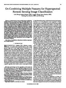
x

N1

[1, 3]

y

N2

x

[1, 9]

[1, 9] SQR

N3

×

4

1

N4

SQRT N5

3

-2

N1(3)

[1, 3]

2

[1, 27] SQR

N3(2)

+

[1, 3]

×

4

1

[-inf, 9]

N4(2)

SQRT N5(2)

3

-2

2

1

+

N6

N2(3)

[1, 9]

1 [0, 0]

y

5

+

N7

[0, 0]

+

N6(1)

N7(1)

[9, 9]

G

G

(a)

(b)

G(0)

Fig. 1. The DAG representation (a) before and (b) after interval evaluations

Following the approach in [20], we use a directed acyclic multigraph, whose edges are totally ordered and whose vertices are ordered by an order in Theorem 1, to represent a constraint system, we therefore call it a Directed Acyclic Graph (DAG). In a DAG, every node represents an elementary operation such as +, ×, ÷, log, exp, . . . and every edge represents the computational flow associated with a coefficient. The ordering of edges is needed for non-communicative operations like the division, and not really necessary for communicative operations. For convenience, a virtual ground node is added to a DAG to be the parent of all the nodes representing the constraints. The reason that we use multigraphs instead of simple graphs for the representation is the fact that some n-ary operations can take the same input more than once, for example, when the expression xx is represented by the operation xy . Example 1. The DAG representation of the following constraint system  2 √  x − 2xy + y = 0, √ 4x + 3xy + 2 y ≤ 9  x ∈ [1, 3], y ∈ [1, 9] is given in Figure 1. {N1 , N2 , N3 , N4 , N5 , N6 , N7 } is an ordering of the nodes satisfying Theorem 1.

3 3.1

Combination Scheme for Constraint Propagation Generalization of Inclusion Concepts

We generalize the concepts related to inclusion function as follows. Definition 5 (Inclusion Representation). Given a set A. A couple I = (R, µ), where R is a set of representing objects and µ is a function from R to 2A , is called an inclusion representation of A if there exists a surjective function ρ : 2A → R such that ∀S ⊆ A : S ⊆ µ(ρ(S)). In this case, ρ is called the representing function of I and µ is called the evaluating function of I.

6

X.-H. Vu, D. Sam-Haroud and B. Faltings

Let I = (R, µ) be an inclusion representation of R. We call I a real inclusion representation of R if each representing object T ∈ R is a tuple consisting of real constants, and the evaluating function µ can be defined by µ(T ) ≡ {fT (VT ) | VT ∈ DT }

(6)

where fT is a real-valued function (with T as a tuple of parameters) and VT is a finite sequence of variables taking values in real domains DT . The representation (6) is called a real representation of µ. It is easy to see that the interval form (1) is a real inclusion representations of R, where each representing object T ∈ R is a couple of reals (a, b), VT = (x), fT is an identity function, and µ is defined by µ(T ) ≡ {x | x ∈ [a, b]}

(7)

The affine form (3) is also a real inclusion representation of R, where each representing object is a tuple T = (x0 , . . . , xn , 1, . . . , n),1 and VT = (ε1 , . . . , εn ) are the variables of the linear function fT (ε1 , . . . , εn ) = x0 + x1 ε1 + . . . + xn εn . Hence, the real representation of the evaluating function is defined by µ(T ) ≡ {x0 + x1 ε1 + . . . + xn εn | (ε1 , . . . , εn ) ∈ [−1, 1]n }

(8)

Definition 6 (Inclusion Function). Given two sets X, Y and a function f : X → Y . Let I X = (RX , µX ) and I Y = (RY , µY ) be two inclusion representations of X and Y , respectively. A function F : RX → RY is called an inclusion function of f , if ∀S ⊆ X, ∀T ∈ RX : S ⊆ µX (T ) ⇒ {f (x) | x ∈ S} ⊆ µY (F (T )). Definition 7 (Inclusion Converter). Let I 1 = (R1 , µ1 ) and I 2 = (R2 , µ2 ) be two inclusion representations of the same set. A function c : R1 → R2 is called an inclusion converter from I 1 to I 2 if ∀S ∈ R1 : µ1 (S) ⊆ µ2 (c(S)). Theorem 2. Let I X = (RX , µX ), I Y = (RY , µY ) and I Z = (RZ , µZ ) be inclusion representations of three sets X, Y and Z, respectively. If F : RX → RY and G : RY → RZ are inclusion functions of two functions f : X → Y and g : Y → Z respectively, then the composite function G ◦ F is an inclusion function of the composite function g ◦ f . Corollary 1. Let I = (R, µ) be an inclusion representation of R. If all elementary operations defined on R are inclusion functions of their counterparts on R, then all factorable functions built on R are also inclusion functions of their counterparts on R. The proof of Theorem 2 follows directly from Definition 5 and Definition 6. Corollary 1 is a straightforward consequence of Theorem 2. The elementary operations in interval arithmetic and affine arithmetic are inclusion functions of their real-valued counterparts, therefore, as a result of Corollary 1, all the factorable operations/functions defined in interval arithmetic (or affine arithmetic) are also inclusion functions of their real-valued counterparts. 1

In implementation, only non-zero coefficients and their indices should be stored.

A Combination Scheme for Numerical Constraint Propagation

3.2

7

A General Combination Scheme

In this section, we describe a general combination scheme that combines the strength of different real inclusion representations for constraint propagation. In this scheme, the input constraint system is represented by a DAG as described in Section 2.3. The data stored at each node, N, of the DAG consist of a representing object for each real inclusion representation I = (R, µ) of R and a constrained range τ (N) ⊆ R often be an interval. We denote by R(N) the representing object (in I) stored at N. Definition 8 (Inclusion Constraint System, ICS). Let (R, µ) be a real inclusion representation of R defined by (6), N a node of a DAG representing a constraint system. The inclusion constraint system induced by a representing object T ≡ R(N) and a constrained domain D ⊆ R is defined by ½ {var(N) ∈ DT , var(N) ∈ D}(var(N) ≡ VT ) if fT is identity, ICS(T, D) ≡ {fT (VT ) = var(N), VT ∈ DT , var(N) ∈ D} otherwise; where var(N) (i.e. the representing variable of N) and the variables in VT are the variables of the constraint system. From (7) and (8) we can see that constructing the inclusion constraint system induced by a representing object and a constrained range [a, b] ⊆ R for interval form and affine form is trivial. Definition 9 (NEV, PCS). Let N be a node of a DAG representing a constraint system, {Ci }ki=1 the children of N, f : Rk → R the elementary operation represented by N, S a finite set of real inclusion representations. The following constraint system is called the pruning constraint system in S at N: PCS(N, S) ≡  V k  if N is ground,  {½ i=1 ICS(R(Ci ), τ (Ci ))} ¾ f (var(C1 ), . . . , var(Ck )) = var(N) ∧ Vk  V otherwise.  i=1 ICS(R(Ci ), τ (Ci ))) (R,µ)∈S (ICS(R(N), τ (N)) ∧ For each I = (R, µ) ∈ S, let fI : Rk → R be an inclusion function of f . The following assignment½is called the node evaluation in I at N (if N 6= ground): ¾ R(N) := R(N) ∩ τ (N) ∩ fI (R(C1 ), . . . , R(Ck )); NEV(N, I) ≡ τ (N) := τ (N) ∩ µ(R(N)); Definition 10 (Pruning Technique). A solution technique is called a pruning technique for a real constraint system if it is capable of reducing some domains of the variables in that system. Let G be a DAG representing the input constraint system. The following algorithm scheme, called CIRD, uses two waiting lists. The first waiting list stores the nodes waiting for evaluation, denoted by Le . The second waiting list stores the nodes waiting for node pruning, denoted by Lp . Note that each node can appear once at a time in a waiting list. The set of real inclusion representations for use in the scheme is denoted by E. Each real inclusion representation in E provides the elementary operations that are inclusion functions of their realvalued counterparts. The following gives the main steps of the CIRD scheme.

8

X.-H. Vu, D. Sam-Haroud and B. Faltings A Scheme for Combining Inclusion Representations on DAG (CIRD) 1. Initialization Phase. (a) Initial Node Evaluation. Select an algorithm for visiting DAGs in an ordering described in Theorem 1. When visiting a node N ∈ G, perform the node evaluation NEV(N, I) for each I ∈ E. (b) Initialize Waiting Lists. Set Le := ∅, Lp := {the list of all nodes representing the active constraints together with all the real inclusion representations of E}. 2. Propagation Phase. Repeat this step until both Le and Lp become empty, or the limit on the number of iterations is reached. (a) Get The Next Node. Select a strategy for getting a node N (and the set S of real inclusion representations associated with N in the corresponding list) from the two waiting lists Le and Lp . (b) Node Evaluation. Do this step only if N was taken from Le at Step 2a. For each I = (R, µ) ∈ S do the following steps:2 i. Perform the node evaluation NEV(N, I). If this returns an empty set, the algorithm stops with an infeasible status. ii. If the changes of R(N) and τ (N) at Step 2(b)i are considered enough to reevaluate the parents of N, then put each node in parents(N) (associated with I) into Le , if N is not the ground node, or into Lp otherwise. iii. If the changes of R(N) and τ (N) at Step 2(b)i are considered enough to do a node pruning at N again, then put (N, I) into Lp . (c) Node Pruning. Do this step only if N was taken from Lp at Step 2a. i. Select a subset T ⊆ S such that for each I ∈ T there are efficient pruning techniques for the constraint system PCS(N, I). ii. Partition T into subsets such that for each subset U of the partition there is a pruning technique that may efficiently reduce the domains of the variables of the system (or a subsystem of) PCS(N, U). After that, apply the associated pruning technique to each system (or a subsystem of) PCS(N, U ) in a certain order. If this process returns an empty set, the algorithm stops with an infeasible status. iii. Let K be the set of all the nodes whose evaluating functions in form (6) contain some variables whose domains were reduced at Step 2(c)ii. Select a subset H of K, for example, such that each node M in H is a descendant of N. For each real inclusion representation I = (R, µ) ∈ H such that the representation of µ(R(M)) in form (6) contains some variables whose domains were reduced at Step 2(c)ii, update R(M) using those newly reduced domains, then update τ (M) := τ (M) ∩ µ(R(M)). If empty is obtained, the algorithm stops with an infeasible status. A. If the changes of R(M) and τ (M) are considered enough to re-evaluate M’s parents, put each node in parents(M) associated with I into Le . B. If the changes of R(M) and τ (M) are considered enough to do a node pruning at M, put (M, I) into Lp .

2

Combining several inclusion representations for better evaluation by using inclusion converters is also an option to try.

A Combination Scheme for Numerical Constraint Propagation

4

9

Specific Combination Strategies as Instances of CIRD

In the rest of the paper, we denote by bEc (resp. dEe) some lower approximation (reps. some upper approximation) in F of the expression E such that bEc ≤ E (resp. E ≤ dEe). We use the notion E = hEi ± e to mean that hEi is an approximation in F of E, and the corresponding bound on the absolute rounding error is e, that is hEi−e ≤ E ≤ hEi+e. Readers are referred to [17] for some rounding techniques in floating-point arithmetic on simple elementary operations. 4.1

Modifications To Affine Arithmetic

Revised Affine Form. One of the limits of the standard affine arithmetic is that the number of noise symbols grows gradually during the computation and the computation cost heavily depends on this number. Inspired by the ideas in [18], [5] and [6], we use a revised affine form similar to (5) but the new term zk εk is replaced by a non-negative accumulative error [−ez , ez ] which represents the maximum absolute error zk of non-affine operations. In other words, the revised affine form of a real-valued quantity x ˆ is defined by x ˆ = x0 + x1 ε1 + . . . + xn εn + ex [−1, 1]

(9)

which consists of two separated parts: the standard affine part of length n, and the interval part. Where the magnitude of the accumulative error, ex ≥ 0, is represented by the interval part. That is, for each value x of the quantity x ˆ (say x ∈ x ˆ), there exist εx ∈ [−1, 1], εi ∈ [−1, 1] (i = 1, . . . , n) such that x = x0 + x1 ε1 + . . . + xn εn + ex εx . We then say it is of length n. The affine operations are now defined by zˆ ≡ αˆ x +β yˆ +γ = (αx0 +βy0 +γ)+

n X

(αxi +βyi )εi +(|α|ex +|β|ey )[−1, 1] (10)

i=1

Therefore, during the computation the length of revised affine forms will not exceed the number of noise symbols at the beginning, i.e. the number of variables of the input constraint system. In rigorous computing, ez will be used to accumulate the rounding errors in floating-point arithmetic, namely (10) can be interpreted as follows z0 = hαx0 +βy0 +γi±e0 , zi = hαxi +βyi i±ei , ez = d|α|ex +|β|ey +

n X

ei e (11)

i=0

Another limit of the standard affine form is that it is not capable of handling half-lines of the form (−∞, a] and [a, +∞), while this is important for many computation methods, especially constraint propagation and search techniques. Hence, we propose to associate each quantity x ˆ with a data field x∞ ∈ {−1, 0, +1}. The revised affine form is then interpreted as follows:3 3

For simplicity, we allow zero coefficients in the formulae in the paper, however in implementation one should keep only nonzero coefficients.

10

X.-H. Vu, D. Sam-Haroud and B. Faltings

 (−∞, +∞)    (−∞, x0 ] x ˆ= [x0 , +∞)    x0 + x1 ε1 + . . . + xn εn + ex [−1, 1]

if ex = +∞, if x∞ = −1, if x∞ = +1, otherwise.

(12)

In an operation, if the domain of a variable is unbounded, i.e. in the first three cases of (12), the other variables are converted into interval forms for that operation performed in interval arithmetic, then the result is converted back to affine form. Therefore, in the rest of paper, we only need to discuss about the last case of (12). The set of all objects in revised affine form is denoted by A. Unary Operations. We give the following theorem as a basis for finding affine approximations of elementary univariate functions in a rigorous manner. Theorem 3 (Affine Approximation of Univariate Functions). Let f be a differentiable function on [a, b], where a < b in R, and dα (x) ≡ f (x) − αx. 1. (a) If ∀x ∈ [a, b] : α ≥ f 0 (x), then ∀x ∈ [a, b] : αx + dα (b) ≤ f (x) ≤ αx + dα (a). (b) If ∀x ∈ [a, b] : α ≤ f 0 (x), then ∀x ∈ [a, b] : αx + dα (a) ≤ f (x) ≤ αx + dα (b). 2. If f 0 is continuous and monotone increasing on [a, b], we have (a) ∀α ∈ [f 0 (a), f 0 (b)], ∃c ∈ [a, b] : f 0 (c) = α. (b) Let g : R → R be a function such that g(α) = dα (c), then ∀x ∈ [a, b] : αx + g(α) ≤ f (x) ≤ αx + max{dα (a), dα (b)}. 3. If f 0 is continuous and monotone decreasing on [a, b], we have (a) ∀α ∈ [f 0 (b), f 0 (a)], ∃c ∈ [a, b] : f 0 (c) = α. (b) Let g : R → R be a function such that g(α) = dα (c), then ∀x ∈ [a, b] : αx + min{dα (a), dα (b)} ≤ f (x) ≤ αx + g(α). Proof. We give the proofs for the case 1a and case 2. The proofs are similar for the other cases. Considering the case 1a, we have f (x) − (αx + dα (b)) = (f (x) − f (b)) − α(x − b) = f 0 (ξ)(x − b) − α(x − b) | for some ξ ∈ [x, b] (Mean Value Theorem) = (x − b)(f 0 (ξ) − α) ≥ 0 | x ≤ b, f 0 (ξ) ≤ α Analogously, we have f (x) − (αx + dα (a)) ≤ 0. The proof of the case 1a therefore follows these results. We now prove the case 2a: because α ∈ [f 0 (b), f 0 (a)] and f 0 is continuous on [a, b] then there exists c ∈ [a, b] as required. Hereafter, we give the proof of the case 2b. For all x ∈ [a, b] we have f (x) − (αx + g(α)) = (f (x) − f (c)) − α(x − c) = f 0 (ξ)(x − c) − α(x − c) | ξ ∈ [x, c] or ξ ∈ [c, x] (Mean Value Theorem) = (x − c)(f 0 (ξ) − f 0 (c)) | α = f 0 (c) ≥0 | ξ is between x and c, f 0 is monotone increasing Moreover, if x ∈ [a, c], we have f (x) − (αx + dα (a)) = (f (x) − f (a)) − α(x − a) = f 0 (η)(x − a) − α(x − a) | for some η ∈ [a, x] (Mean Value Theorem) = (x − a)(f 0 (η) − f 0 (c)) | α = f 0 (c) ≤0 | η ≤ c, f 0 is monotone increasing

A Combination Scheme for Numerical Constraint Propagation

11

Table 1. Examples of functions f ∈ C 1 ([a, b]) satisfying the conditions of Theorem 3 f (x) [a, b] is a subset of 2 x (−∞, +∞) √ x [0, +∞) x e (−∞, +∞) log x (0, +∞) xn : n ≥ 2 is even (−∞, +∞) xn : n ≥ 3 is odd (−∞, 0] xn : n ≥ 3 is odd [0, +∞) 1/xn : n ≥ 2 is even (−∞, 0); (0, +∞) 1/xn : n ≥ 1 is odd (−∞, 0) 1/xn : n ≥ 1 is odd (0, +∞) xr : r ∈ / [0, 1] (0, +∞) xr : r ∈ (0, 1) (0, +∞)

f 0 (x) 2x √ 1/(2 x) ex 1/x nxn−1 nxn−1 nxn−1 −n/xn+1 −n/xn+1 −n/xn+1 rxr−1 rxr−1

f0 ↑ ↓ ↑ ↓ ↑ ↓ ↑ ↑ ↓ ↑ ↑ ↓

g(α) −α2 /4 1/(4α) : α > 0 α(1 − log α) : α > 0 −(1 + log α) p: α > 0 (1 − n)pn−1 (α/n)n n (n − 1) n−1 p(α/n) : α ≥ 0 n : α ≥ 0 (1 − n) n−1 (α/n) p n+1 (n + 1) p (−α/n)n n −(n + 1) n+1 p (−α/n) : α < 0 (n + 1) n+1 (−α/n)n : α < 0 (1 − r)(α/r)(r/(r−1)) : αr > 0 (1 − r)(α/r)(r/(r−1)) : α > 0

Similarly, if x ∈ [c, b] we have f (x) − (αx + dα (b)) ≤ 0. Hence, we have f (x) ≤ αx + max{dα (a), dα (b)} for all x ∈ [a, b]. The proof is then completed. ¤ To illustrate the usefulness of Theorem 3, in Table 1 we give the functions f 0 and g for some elementary functions, and in Figure 2 we give a procedure to find a safe Chebyshev affine approximation of a function f ∈ C 1 ([a, b]) such that f 0 is monotone, when given the function g satisfying the conditions in Theorem 3. Proposition 1. Let αˆ x + β + δ[−1, 1] be the revised affine form produced by the procedure in Figure 2, where [a, b] is the range of x ˆ. Suppose that f ∈ C 1 ([u, v]) 0 and f is monotone on [u, v], where [u, v] ⊇ [a, b] such that f 0 (v) ≥ df 0 (b)e if f 0 is monotone increasing, or f 0 (u) ≥ df 0 (a)e if f 0 is monotone decreasing. We have ∀x ∈ x ˆ : f (x) ∈ αˆ x + β + δ[−1, 1]. Proof. Following the Mean Value Theorem, there is some c∗ ∈ [a, b] such that α∗ = f 0 (c∗ ) = (f (b) − f (a))/(b − a) Therefore α∗ ≤ d(df (b)e − bf (a)c)/(b − a)e = α ⇒ α ≥ min{f 0 (a), f 0 (b)} (f 0 is monotone) Hereafter, we prove for the case f 0 is monotone increasing, the proof for the other case is similar. If α > df 0 (b)e, then ∀x ∈ [a, b] : α > f 0 (x). Hence, following the case 1a of Theorem 3, we have, for all x ∈ [a, b] αx + dα (b) ≤ f (x) ≤ αx + dα (a) ⇒ αx + dmin ≤ αx + dα (b) ≤ f (x) ≤ αx + dα (a) ≤ αx + dmax If α ≤ f 0 (b), the result follows directly from the case 2 of Theorem 3. In the rest of the proof, we consider the case f 0 (b) < α ≤ df 0 (b)e. Similar to the above, we have αx + dα (b) ≤ f (x) ≤ αx + dα (a). Moreover, applying the case 2 of Theorem 3 to [b, v], we have x ∈ [b, v] : αx + g(α) ≤ f (x) ⇔ x ∈ [b, v] : g(α) ≤ f (x) − αx ⇒ g(α) ≤ f (b) − αb = dα (b)

12

X.-H. Vu, D. Sam-Haroud and B. Faltings

procedure AffineApproximation(in : x ˆ, f ∈ C 1 ([a, b]), f 0 , g; out : αˆ x + β + δ[−1, 1]) fa := bf (a)c; fb := df (b)e; α := d(fb − fa )/(b − a)e; if f 0 is monotone increasing on [a, b] then da := df (a)e − bαac; if α > df 0 (b)e then dmin := bf (b)c − dαbe; dmax := da ; else dmin := bg(α)c; dmax := max{da , fb − bαbc}; end-if else-if f 0 is monotone decreasing on [a, b] then db := bf (b)c − dαbe; if α > df 0 (a)e then dmin := db ; dmax := df (a)e − bαac; else dmin := min{fa − dαae, db }; dmax := dg(α)e; end-if end-if β := midpoint([dmin , dmax ]); δ := radius([dmin , dmax ]); end Fig. 2. This is a procedure to find a Chebyshev affine approximation of a function f ∈ C 1 ([a, b]) such that f 0 is monotone, when given the function g in Theorem 3

Therefore, for all x ∈ [a, b] we have αx + g(α) ≤ f (x) ≤ αx + dα (a) = max{αx + dα (a), αx + dα (b)} ⇒ αx + dmin ≤ f (x) ≤ αx + dmax As a result, ∀x ∈ x ˆ : f (x) ∈ αˆ x + β + δ[−1, 1]. The proof is then completed. ¤ Readers are referred to Section 2 of [21] for a method to compute affine approximations of non-differentiable functions. Multiplication. Similar to the product of two G intervals in [5] and [6], the product of two revised affine forms x ˆ and yˆ of length n is another revised affine form zˆ of length n defined as follows n X z0 = x0 y0 + 0.5 xi yi , zi = x0 yi + y0 xi (i = 1, . . . , n) (13) i=1

ez = ex ey + ey

n X i=0

|xi | + ex

n X i=0

|yi | +

n X i=1

|xi |

n X i=1

|yi | − 0.5

n X

|xi yi |

(14)

i=1

This is similar to, but tighter than, the formula for multiplication in [6] when exactly porting into revised affine form. The time complexity of (10) and (14) is O(n). In rigorous computing, we use the following computations. n n X X u=d |xi |e, v = d |yi |e (15) i=1

i=1

A Combination Scheme for Numerical Constraint Propagation

z0 = hx0 y0 + 0.5

n X

xi yi i ± e0 , zi = hx0 yi + y0 xi i ± ei (i = 1, . . . , n)

13

(16)

i=1

ez = dex ey + ey (|x0 | + u) + ex (|y0 | + v) + uv +

n X

ei e − b0.5

i=0

n X

|xi yi |c (17)

i=1

Proposition 2. The affine multiplication function defined by {(13), (14)} or by {(15), (16), (17)} is an inclusion function of the real multiplication. Proof. It suffices to prove that ∀x ∈ x ˆ, y ∈ yˆ : xy ∈ zˆ = z0 + By definition, there exist ex , ey ∈ [−1, 1] such that x = x0 +

n X i=1

xi εi + ex εx , y = y0 +

n X

Pn

i=1 zi εi +ez [−1, 1].

yi εi + ey εy

i=1

Therefore, weP have n xy = x0 yP + xi y0 )εi + x0 eyP εy + y0 ex εx + ex ey εxP εy + 0 i=1 (x0 yi +P n n n n ey i=1 xi εy εi + ex i=1 yi εx εi + i,j=1;i6=j xi yj εi εi + i=1 xi yi ε2i Pn ∈ x0 yP 0 )εi + |x0 |ey [−1, 1] 0+ i=1 (x0 yi + xi yP P+n |y0 |ex [−1, 1] + ex ey [−1, 1]+ n n ey i=1 |xi |[−1, 1] + ex i=1 |yi |[−1, 1] + i,j=1;i6=j |xi yj |+ Pn yi + |xi yi |[−1,P 1]) 0.5 i=1 (xiP n n = (x0 y0 + 0.5P i=1 xi yi ) + Pi=1 (x0 yi +Pxi y0 )εi +P[−1, 1]× Pn n n n n (ex eyP + ey i=0 |xi | + ex i=0 |yi | + i=1 |xi | i=1 |yi | − 0.5 i=1 |xi yi |) n ⊆ z0 + i=1 zi εi + ez [−1, 1] = zˆ (Follow {(13), (14)} or {(15), (16), (17)}). ¤ Division. In our implementation, we compute the quotient zˆ = x ˆ/ˆ y by rewriting it as x ˆ × (1/ˆ y ). However, it is worth mention that in [6] and [22], the authors have proposed better methods for division that have some interesting properties such as x ˆ/ˆ x = 1. 4.2

New Combination Strategies for Constraint Propagation

In the rest, we will abuse the notions I and A to denote the real inclusion representations, (I, µI ) and (A, µA ), defined on interval arithmetic and revised affine arithmetic, respectively; where the function µI is defined by (7) and the function µA follows (12). In general, the performance of a propagator following the CIRD scheme depends on the design of each step in the scheme. In this section, we propose some simple strategies for each step in the CIRD scheme using the two inclusion representations, I and A. Combining different strategies at all the steps makes different combination strategies for constraint propagation. Step 1a: Initial Node Evaluation. A post-order visiting or a recursive evaluation starting from the ground node is an option for the visit at Step 1a.

14

X.-H. Vu, D. Sam-Haroud and B. Faltings

procedure NodeLevel(in : DAG) Initialize the level of each node to zero. for each visit in pre-order going from a parent P to its children N do level(N) := max{level(N), level(P) + 1}; end Fig. 3. This is a procedure assigning a node level to each node in a DAG.

Step 2a: Get The Next Node. At first, we assign a node level to each node in the DAG representing the constraint system such that each ancestor has a lower level than that of their descendants, hence, an ordering in Theorem 1 can be obtained easily. Figure 3 gives a simple procedure for this purpose. Lp is sorted in the ascending order of node levels. It is to maintain that ancestors being taken into pruning processes before their descendants. Le is sorted in the descending order of node levels. It is to sure that descendants being evaluated before their ancestors. There are two simple strategies to get the next node from {Le , Lp }. The first one is to get the next node from Lp whenever it is not empty. The second one is to get the next node from one of the two waiting lists until it becomes empty, then switch to the other list. In our implementation, we use the first simple strategy. More complicated strategies for choosing the next node can be used as alternatives, for example, based on the pruning efficiency of nodes. Step 2b: Node Evaluation. For the node evaluation at each node N, we can perform NEV(N, A) and NEV(N, I) in any order, if N is not the ground node. At Step 2(b)ii, Step 2(b)iii and Step 2(c)iii, we only count on the changes of τ (N) in our current implementation. A change of τ (N) is often considered enough if the ratio of the new width to the old width is less than a number predefined rw ∈ (0, 1) and the difference between the old width and the new width is greater than a predefined number dw > 0 (see [1] for details). More complicated criteria that have been used in constraint programming can be used as alternatives. Step 2c: Node Pruning. The subset T at this step can be chosen as {I, A}. For node pruning, we use PCS(N, {I}) and the following subsystem of PCS(N, {A}):    f (var(C1 ), . . . , var(Ck )) = var(N);  PCS(N, {I}) ≡ var(N) ∈ τ (N); if N is not ground.  Vk  (var(C ) ∈ τ (C )); i i i=1 ( V k { i=1 ICS(A(Ci ), τ (Ci ))} if N is ground, Vk PCSL (N, {A}) ≡ {ICS(A(N), τ (N)) ∧ i=1 ICS(A(Ci ), τ (Ci ))} otherwise,   P  xM,0 + ki=1 xM,i εi + eM εM = var(M);  where ICS(A(M), D) ≡ εi ∈ [−1, 1] (i = 1, . . . , n);   εM ∈ [−1, 1]; var(M) ∈ D;

A Combination Scheme for Numerical Constraint Propagation

15

Example 2. We give the node levels for the example described in Section 2.3 in brackets next to the node names in Figure 1b. At the beginning, we have τ (N1 ) = I(N1 ) = [1, 3]; A(N1 ) = 2 + ε1 τ (N2 ) = I(N2 ) = [1, 9]; A(N2 ) = 5 + 4ε2 τ (Ni ) = I(Ni ) = A(Ni ) = [−∞, +∞] (i = 3, 4, 5) τ (N6 ) = I(N6 ) = [0, 0]; A(N6 ) = 0 τ (N7 ) = I(N7 ) = [−∞, 9]; A(N7 ) = [−∞, 9] After the initial node evaluation, we have the following changes: τ (N3 ) = I(N3 ) = [1, 9]; A(N3 ) = 4.5 + 4ε1 + 0.5[−1, 1] τ (N4 ) = I(N4 ) = [1, 27]; A(N4 ) = 10 + 5ε1 + 8ε2 + 4[−1, 1] τ (N5 ) = I(N5 ) = [1, 3]; A(N5 ) = 2.125 + ε2 + 0.125[−1, 1] τ (N6 ) = I(N6 ) = [0, 0]; A(N6 ) = −13.375 − 6ε1 − 15ε2 + 8.625[−1, 1] τ (N7 ) = I(N7 ) = [9, 9]; A(N7 ) = 42.25 + 19ε1 + 26ε2 + 12.25[−1, 1] Denoting the variable var(Ni ) by vi , we have, for example, PCS(N6 , {A}) ≡ PCS(N6 , {I}) ∧ PCSL (N6 , {A}) where

½ PCS(N6 , {I}) ≡

and

v3 − 2v4 + v5 = v6 v3 ∈ [1, 9]; v4 ∈ [1, 27]; v5 ∈ [1, 3]; v6 ∈ [0, 0]

 4.5 + 4ε1 + 0.5εN3 = v3     10 + 5ε1 + 8ε2 + 4εN4 = v4    2.125 + ε2 + 0.125εN5 = v5 PCSL (N6 , {A}) ≡ −13.375 − 6ε1 − 15ε2 + 8.625εN6 = v6    6  (ε  1 , ε2 , εN3 , εN4 , εN5 , εN6 ) ∈ [−1, 1]   v3 ∈ [1, 9]; v4 ∈ [1, 27]; v5 ∈ [1, 3]; v6 ∈ [0, 0]

Backward Propagation. If N is not the ground, the domains of the variables of the constraint system PCS(N, {I}) can be pruned by a pruning technique which is called backward propagation in [1] and [20]. In brief, let f be the elementary operation represented by a node N, we then have the relation var(N) = f ({var(Ci )}ki=1 ). For each i in {1, . . . , k}, the backward propagation computes a cheap evaluation of the i-th projection of the relation var(N) = f ({var(Ci )}ki=1 ) onto var(Ci ). In case there exist a function gi : Rk → R such that we can write var(Ci ) = gi (var(N), {var(Cj )}kj=1;j6=i ). Let Gi be an inclusion function of gi in I. In this case, the backward propagation at N is defined by I(Ci ) := I(Ci ) ∩ Gi (I(N), {I(Cj )}kj=1;j6=i ) (i = 1, . . . , k) (18) For instance, in Example 2 we have v6 = f (v3 , v4 , v5 ) with f (x, y, z) = x−2y +z. Hence, we can write v3 = g1 (v6 , v4 , v5 ), v4 = g2 (v6 , v3 , v5 ), v5 = g3 (v6 , v3 , v4 ); where g1 (x, y, z) = x+2y−z, g2 (x, y, z) = (−x+y+z)/2, g3 (x, y, z) = x−y+2z. In another case often seen in practice, f is a univariate function (i.e. k = 1), we can use the backward propagation defined by I(C1 ) := I(C1 ) ∩ f −1 (I(N)), where f −1 (.) denotes the reciprocal image. After the backward propagation, at Step 2(c)iii we only need to consider k nodes H = {Ci | i = 1, . . . , k} for update and for putting into the waiting lists.

16

X.-H. Vu, D. Sam-Haroud and B. Faltings

Affine Pruning. In A, each variable of the input constraint system is associated with one noise symbol εi (i = 1, . . . , n). The system PCSL (N, {A}) is a linear constraint system, therefore, the domains of the variables of PCSL (N, {A}) can be pruned by using a safe linear programming technique [23]. If the operation represented by N is linear, we can apply a safe linear programming technique to PCS(N, {A}), instead of PCSL (N, {A}), to get tighter bounds on the variables. For efficiency, only the domains of the variables {var(Ci )}ki=1 and/or {εi }ni=1 are needed to be pruned. We can devise three possible pruning strategies for Step 2(c)iii. The first strategy only requires to prune the domains of {var(Ci )}ki=1 , after that, considers the update for H = {Ci }ki=1 . The second strategy only requires to prune the domains of {εi }ni=1 . The third strategy is to prune the domains of both {var(Ci )}ki=1 and {εi }ni=1 . For the last two strategies, the set H can be chosen as any subset of the set of N’s descendants whose noise variables in µA have just been pruned. In our implementation, we use the second pruning strategy with two options for H: the set of N’s descendants or the set of variables associated with εi (i = 1, . . . , n). If for each i ∈ {1, . . . , n} the new domain of noise variable εi is [ai , bi ] ⊆ [−1, 1], then the range update at M ∈ H will be n X τ (M) := τ (M) ∩ (xM,0 + xM,i [ai , bi ] + eM [−1, 1]) (19) i=1

The cost of linear programming is expensive, therefore, we should use the affine pruning technique only if the pruning ratio is high. We propose to use the affine pruning technique only if the accumulative error eM of each node M involving the above linear systems is small enough, that is, the range Pn of the operation at M lies in a thin slot between two hyperplanes x + M,0 i=1 xM,i εi − eM and Pn xM,0 + i=1 xM,i εi + eM in the space of the noise variables (ε1 , . . . , εn ). The combination of backward propagation and affine pruning techniques makes different strategies for node pruning in the CIRD scheme.

5

Experiments

Comparison with Linearization-based Techniques. The first technique to compare with is a recent mathematical technique, A2, in [6] which was specially designed to solve non-linear equation systems. It converts the equation system into separable form then uses affine arithmetic to enclose the system by a linear relaxation system {L(x, y) = Ax + By + b, x ∈ x, y ∈ y}, where A and B are real matrices, and b is a real vector. This technique has to assume a posteriorcondition that A is invertible. No rigorous rounding technique is found in [6]. We take the example used for illustrating the power of A2 in [6] for the comparison:  ((4x3 + 3x6 )x3 + 2x5 )x3 + x4 = 0,     ((4x2 + 3x6 )x2 + 2x5 )x2 + x4 = 0     ((4x  1 + 3x6 )x1 + 2x5 )x1 + x4 = 0,   x4 + x5 + x6 = 0 (((x2 + x6 )x2 + x5 )x2 + x4 )x2 + (((x3 + x6 )x3 + x5 )x3 + x4 )x3 = 0     (((x  1 + x6 )x1 + x5 )x1 + x4 )x1 + (((x2 + x6 )x2 + x5 )x2 + x4 )x3 = 0     x ∈ [0.0333, 0.2173], x2 ∈ [0.4000, 0.6000], x3 ∈ [0.7826, 0.9666] 1   x4 ∈ [−0.3071, −0.1071], x5 ∈ [1.1071, 1.3071], x6 ∈ [−2.1000, −1.9000]

(20)

A Combination Scheme for Numerical Constraint Propagation

17

Table 2. Comparison between Quad and CIRD1: time is in seconds; #It is the number of iterations; #Box is the number of boxes in output. The cells are filled with “n/a” if results are not yet available for comparison in this submission, due to our limited access to the code of Quad. Problem Gough-Steward Yama196 [n = 30] Yama196 [n = 60] Yama196 [n = 100] Yama196 [n = 200] Yama196 [n = 300]

Quad CIRD1 Time Ratio #It #Box Time (s) CPU speed #It #Box Time (s) CPU speed Quad/CIRD1 24 4 183.0 1.0 GHz 912 4 9.9 800 MHz 23.1 108 16 31.4 2.66 GHz 25 2 8.5 2.0 GHz 4.9 n/a n/a n/a n/a 18 2 50.0 2.0 GHz n/a n/a n/a n/a 20 2 194.8 2.0 GHz n/a n/a n/a n/a 20 2 1305.5 2.0 GHz n/a n/a n/a n/a 20 2 4580.6 2.0 GHz

The system (20) is known to have an unique solution. To solve (20) at the resolution 10−5 using a bisection search, A2 has to perform 917 iterations in 3.46 seconds on a 1.7 GHz Pentium PC to reduce the problem to 5 boxes (see [6]); while an instance of our scheme, called CIRD1, has to perform 54 iterations in only 0.25 seconds on a 2.0 GHz Pentium PC to reduce the problem to 3 boxes. Hence, CIRD1 is about 11.7 times faster than A2 for the system (20), while it is more rigorous and accurate than A2. Another technique to compare with is a very recent filtering technique called Quad in [3], which was specifically designed to address quadratic constraints and an extension of Quad in [4]. We take two problems, Gough-Steward and Yama196, from [3] and [4] respectively for comparison. Gough-Steward is a 9dimensional quadratic equation system in Robotics having four solutions [3]. There is probably a typo mistake at the third term in the fourth equation of Gough-Steward in [3], that should be corrected to z2 z3 as follows (otherwise, the problem will have no solution).  2 x1 + y12 + z12 = 31    x2 + y 2 + z 2 = 39   2 2 2    x23 + y32 + z32 = 29     x1 x2 + y1 y2 + z1 z2 + 6x1 − 6x2 = 51     x1 x3 + y1 y3 + z1 z3 + 7x1 − 2y1 − 7x3 + 2y3 = 50    x2 x3 + y2 y3 + z2 z3 + x2 − 2y2 − x3 + 2y3 = 34 −12x1 + 15y1 − 10x2 − 25y2 + 18x3 + 18y3 = −32     −14x1 + 35y1 − 36x2 − 45y2 + 30x3 + 18y3 = 8     2x  1 + 2y1 − 14x2 − 2y2 + 8x3 − y3 = 20     x1 ∈ [−2.00, 5.57], y1 ∈ [−5.57, 2.70], z1 ∈ [0.00, 5.57]     x ∈ [−6.25, 1.30], y2 ∈ [−6.25, 2.70], z2 ∈ [−2.00, 6.25]   2 x3 ∈ [−5.39, 0.70], y3 ∈ [−5.39, 3.11], z3 ∈ [−3.61, 5.39]

(21)

Yama196 is a series of high dimensional problems consisting of n variables and n equations of form {(n + 1)2 xi−1 − 2(n + 1)2 xi + (n + 1)2 xi+1 + exi = 0, xi ∈ [−10, 10] | i = 1, . . . , n}, where x0 = xn+1 = 0. Similar to [4], we use the resolution 10−8 for these problems. Table 2 gives the comparison between CIRD1 and Quad (at the same resolution) for the above two problems whose results has been reported in [3] and [4]. Comparison with Interval Propagation Techniques. We have carried out experiments on CIRD1 and two other recent interval propagation techniques. The

18

X.-H. Vu, D. Sam-Haroud and B. Faltings

first one is the Box Consistency in ILOG Solver 6.0, denoted by BOX. The second one is called HC4 (Revised Hull Consistency) in [1]. The experiments are carried out on 33 problems which are unbiasedly selected and divided into 5 test cases. The test case T1 consists of 7 problems with isolated solutions that are solvable by all three propagators. The test case T2 consists of 5 problems with isolated solutions that are solvable by only two propagators. The test case T3 consists of 8 problems with isolated solutions that cause at least two of three techniques being stopped due to timeout or due to running more than 106 iterations. The test case T4 consists of 7 small problems with continuum of solutions that are solvable at resolution 10−2 . The test case T5 consists of 6 hard problems with continuum of solutions that are solvable at resolution 10−1 . The timeout value is 6000 seconds for all the test cases, it will be used as the running time for the techniques which is timeout in the next result analysis (i.e. we are in favor of slow techniques). For the first three test cases, the resolution is 10−4 and the search to be used is bisection. For the last two test cases, the search to be used is a simple search technique, called UCA6, for inequalities (see [7, 8]). The comparison of the interval propagation techniques is based on the measures of 1. The running time: The relative ratio of the running time of each propagator to that of CIRD1 is called the relative time ratio. 2. The number of boxes: The relative ratio of that number of boxes in the output of each propagator to that of CIRD1 is called the relative cluster ratio. 3. The number of iterations: the number of iterations in search needed to solve the problems. The relative ratio of the number of iterations used by each propagator to that of CIRD1 is called the relative iteration ratio. 4. The volume of boxes (only for T1 , T2 , T3 ): We consider the reduction per dimension when replacing the set of output boxes by a volume-equivalent hypercube. The relative ratio of the reduction gained by each propagator to that of CIRD1 is called the relative reduction ratio. 5. The volume of inner boxes (only for T4 , T5 ): The ratio of the volume of inner boxes to the volume of all output boxes is called the inner volume ratio. The overviews of results in our experiments are given in Table 3 and Table 4. Clearly, CIRD1 is superior than BOX and HC4 in performance and quality for the problems with isolated solutions. CIRD1 still outperforms the others for the problems with continuum of solutions while being a little better than the others in quality of the output.

6

Conclusion

In this paper, we propose a novel generic scheme, CIRD, for constraint propagation using different inclusion representations on DAG. The scheme is applicable to most of known inclusion representations, including interval arithmetic, affine arithmetic, polyhedral/quadratic enclosures and their generalizations. The modifications and improvements on the rigorous computations of affine arithmetic are also proposed. As a result, we give several new combination strategies for

A Combination Scheme for Numerical Constraint Propagation

19

Table 3. (a) The average of the relative time ratios is taken over all the problems in the test cases T1 , T2 , T3 ; the averages of the other relative ratios are taken over the problems in the test case T1 , i.e. over the problems which are solvable by all the techniques. (b) The averages of the relative ratios are taken over all the problems in the test cases T4 , T5 . In general, the lower the relative ratio, the better the performance/quality; and the higher the inner volume ratio, the better the quality. (a) Isolated Solutions Propagator CIRD1 BOX HC4

(b) Continuum of Solutions

Relative Relative Relative Relative Relative Inner Relative Relative time reduction cluster iteration time volume cluster iteration ratio ratio ratio ratio ratio ratio ratio ratio

1.000 1687.162 3791.425

1.000 1.000 6.014 10.057 9.102 33.157

1.000 1.000 0.945 3.769 3.414 0.944 5.019 60.101 0.941

1.000 1.102 1.168

1.000 1.056 1.118

Table 4. This table contains the averages of the relative time ratios taken over the problems in each test case. (a) Isolated Solutions (b) Continuum of Solutions Propagator Test case T1 Test case T2 Test case T3 Test case T4 Test case T5 CIRD1 1.00 1.00 1.00 1.00 1.00 BOX 8.35 4848.89 204.25 2.33 4.68 HC4 19.30 11088.74 266.23 31.42 93.56

constraint propagation based on interval arithmetic, affine arithmetic, interval constraint propagation and (safe) linear programming. After all, we show by experiments that one implementation, CIRD1, outperforms recent techniques by 1-4 orders of magnitude in speed, while still being better in quality measures. A direction for near future is to try all the proposed strategies and options in Section 4.2 to investigate different combination strategies using interval arithmetic and affine arithmetic under different settings. Another direction for future is to use the quadratic form/arithmetic in [18] and use quadratic programming techniques (e.g. [3]) in the way similar to the above affine pruning technique. Moreover, developing learning strategies for choosing the next node from the waiting lists based on the pruning efficiency of nodes is another possible way to improve the overall performance of the propagation.

7

Acknowledgments

This research is funded by the European Commission and the Swiss Federal Education and Science Office through the COCONUT project (IST-2000-26063). We would like to thank ILOG for the licenses of ILOG Solver/CPLEX used in the COCONUT project.

References 1. Benhamou, F., Goualard, F., Granvilliers, L., Puget, J.F.: Revising Hull and Box Consistency. In: Proceedings of the International Conference on Logic Programming (ICLP’99), Las Cruces, USA (1999) 230–244

20

X.-H. Vu, D. Sam-Haroud and B. Faltings

2. Jaulin, L., Kieffer, M., Didrit, O., Walter, E.: Applied Interval Analysis. First edn. Springer (2001) 3. Lebbah, Y., Rueher, M., Michel, C.: A Global Filtering Algorithm for Handling Systems of Quadratic Equations and Inequations. In: Proceedings of the 9th International Conference on Principles and Practice of Constraint Programming (CP’2003). Volume LNCS 2470., Springer (2003) 109–123 4. Lebbah, Y., Michel, C., Rueher, M.: Global Filtering Algorithms Based on Linear Relaxations . In: Notes of the 2nd International Workshop on Global Constrained Optimization and Constraint Satisfaction (COCOS 2003), Switzerland (2003) 5. Kolev, L.: Automatic Computation of a Linear Interval Enclosure. Realiable Computing 7 (2001) 17–18 6. Kolev, L.: An Improved Interval Linearization for Solving Non-Linear Problems. In: 10th GAMM - IMACS International Symposium on Scientific Computing, Computer Arithmetic, and Validated Numerics (SCAN2002), France (2002) 7. Silaghi, M.C., Sam-Haroud, D., Faltings, B.: Search Techniques for Non-linear CSPs with Inequalities. In: Proceedings of the 14th Canadian Conference on Artificial Intelligence. (2001) 8. Vu, X.H., Sam-Haroud, D., Silaghi, M.C.: Numerical Constraint Satisfaction Problems with Non-isolated Solutions. In: Global Optimization and Constraint Satisfaction. Volume LNCS 2861., Springer-Verlag (2003) 194–210 9. Kearfott, B.: Interval Computations: Introduction, Uses, and Resources. Euromath Bulletin 2(1) (1996) 95–112 10. Burkill, J.: Functions of Intervals. Proceedings of the London Mathematical Society 22 (1924) 375–446 11. Sunaga, T.: Theory of an Interval Algebra and its Applications to Numerical Analysis. RAAG Memoirs 2 (1958) 29–46 12. Moore, R.: Interval Arithmetic and Automatic Error Analysis in Digital Computing. PhD thesis, Stanford University, USA (1962) 13. Moore, R.: Interval Analysis. Prentice Hall, Englewood Cliffs, NJ (1966) 14. Alefeld, G., Herzberger, J.: Introduction to Interval Computations. Academic Press, New York, NY (1983) 15. Hickey, T., Ju, Q., Van Emden, M.: Interval Arithmetic: from Principles to Implementation. Journal of the ACM (JACM) 48(5) (2001) 1038–1068 16. Comba, J., Stolfi, J.: Affine Arithmetic and its Applications to Computer Graphics. In: Proceedings of SIBGRAPI’93, Brazil (1993) 17. Stolfi, J., de Figueiredo, L.: Self-Validated Numerical Methods and Applications. In: Monograph for 21st Brazilian Mathematics Colloquium (IMPA), Brazil (1997) 18. Messine, F.: Extentions of Affine Arithmetic: Application to Unconstrained Global Optimization. Journal of Universal Computer Science 8(11) (2002) 992–1015 19. Martin, R., Shou, H., Voiculescu, I., Bowyer, A., Wang, G.: Comparison of Interval Methods for Plotting Algebraic Curves. Computer Aided Geometric Design 19(7) (2002) 553–587 20. Schichl, H., Neumaier, A.: Interval Analysis on Directed Acyclic Graphs for Global Optimization (2004) preprint - University of Vienna, Autria. 21. Kolev, L.: A New Method for Global Solution of Systems of Non-Linear Equations. Realiable Computing 4 (1998) 125–146 22. Miyajima, S., Miyata, T., Kashiwagi, M.: A New Dividing Method in Affine Arithmetic. IEICE Transaction on Fundamentals of Electronics, Communications and Computer Sciences E86-A(9) (2003) 2192–2196 23. Neumaier, A., Shcherbina, O.: Safe Bounds in Linear and Mixed-Integer Programming. Mathematical Programming A 99 (2004) 283–296