Attea & Hameed
Iraqi Journal of Science, 2014, Vol 55, No.1, pp:224-240
A Genetic Algorithm for Minimum Set Covering Problem in Reliable and Efficient Wireless Sensor Networks Bara'a A. Attea*, Sarab M. Hameed Department of Computer Science, College of Science, Baghdad University, Baghdad, Iraq. Abstract Densely deployment of sensors is generally employed in wireless sensor networks (WSNs) to ensure energy-efficient covering of a target area. Many sensors scheduling techniques have been recently proposed for designing such energyefficient WSNs. Sensors scheduling has been modeled, in the literature, as a generalization of minimum set covering problem (MSCP) problem. MSCP is a wellknown NP-hard optimization problem used to model a large range of problems arising from scheduling, manufacturing, service planning, information retrieval, etc. In this paper, the MSCP is modeled to design an energy-efficient wireless sensor networks (WSNs) that can reliably cover a target area. Unlike other attempts in the literature, which consider only a simple disk sensing model, this paper addresses the problem of scheduling the minimum number of sensors (i.e., finding the minimum set cover) while considering a more realistic sensing model to handle uncertainty into the sensors' target-coverage reliability. The paper investigates the development of a genetic algorithm (GA) whose main ingredient is to maintain scheduling of a minimum number of sensors and thus to support energy-efficient WSNs. With the aid of the remaining unassigned sensors, the reliability of the generated set cover provided by the GA, can further be enhanced by a post-heuristic step. Performance evaluations on solution quality in terms of both sensor cost and coverage reliability are measured through extensive simulations, showing the impact of number of targets, sensor density and sensing radius. Keywords: Coverage, energy efficiency, genetic algorithm, probabilistic sensing model, SCP, wireless sensor networks.
الخوارزمية الجينية لمشكلة المجموعة االدنى للتغطية في شبكات االستشعار الالسلكية الموثوقة والفعالة
سراب مجيد حميد،براء علي عطيه . العراق، بغداد، جامعة بغداد، كلية العلوم،قسم الحاسبات الخالصة
( لضمانWSNs) يستخدم عادة نشر أجهزة االستشعار بكثافة في شبكات االستشعار الالسلكية
حديثأ تم اقتراح العديد من تقنيات جدولة أجهزة.تغطية كفوءه وأقتصادية في المنطقة المستهدفة كفوء من ناحية استخدام الطاقة وأصبحت هذه المشكل تعميم لمشكلهWSNs االستشعار لتصميم
والمطبقة في حل العديد منNP-Hard هي مشكلةMSCP .(MSCP) المجموعة االدنى للتغطيه . وما إلى ذلك من المشاكل، واسترجاع المعلومات، وتخطيط الخدمة،المشاكل الناجمة مثل التصنيع __________________________________________ *Email:
[email protected] 224
Attea & Hameed
Iraqi Journal of Science, 2014, Vol 55, No.1, pp:224-240
( والتي يمكنWSNs) لتصميم شبكات االستشعار الالسلكيةMSCP تم نمذجة، في هذ البحث
، على عكس محاوالت أخرى في هذا المجال.أن تغطي المنطقة المستهدفة بثقة وبطريقة أقتصادية
يتناول هذا البحث مشكلة جدولة الحد األدنى لعدد من أجهزة االستشعار ( إيجاد الحد األدنى لغطاء في نموذج االستشعار أكثر واقعية للتعامل مع حالة عدم اليقين في موثوقية أجهزة،)مجموعة
( للحفاظ علىGA) تدارس هذا البحث تطوير الخوارزمية الجينية.االستشعار في تغطية الهدف
وبمساعدة من. كفوء في استخدام الطاقةWSNs لدعم،جدوله لعدد أدنى من أجهزة االستشعار بعدGA يمكن زيادة موثوقية تغطية المجموعة التي تقدمها،أجهزة االستشعار غير المعينة المتبقية
تم قياس تقييم األداء على نوعية الحل من حيث تكلفة.خطوة الكشف عن مجريات األمور
وكثافة، والتي تبين أثر عدد األهداف،االستشعار وموثوقية التغطية من خالل محاكاة واسعة النطاق
.اجهزة االستشعار ونصف قطر االستشعار عن بعد
1.Introduction Recently, many applications, ranging from remote harsh field monitoring to surveillance and smart homes, have been directed towards studying and building their backbones based on Wireless sensor networks (WSNs). The dense ad-hoc deployment of such sensors from an aircraft into the monitoring area can results in network configurations with adequate targets coverage level. However, recharging or replacing a sensor’s battery is generally infeasible. Hence, efficient utilization of the limited energy is one of the critical design considerations in WSNs. Energy-aware mechanism has been substantially pursued by the research community in order to form long lived WSNs. Energy saving techniques can generally be classified in the following categories: 1. Energy-efficient data aggregation, gathering and routing; 2. Power management by adjusting the transmission and/or sensing range of sensor nodes; and 3. Sensor wake-up scheduling to alternate between active and idle state. In this paper, we will consider the third approach to design energy-efficient WSNs while completely monitoring the targets. In this class of techniques, sensor activities are scheduled into disjoint set covers (DSC), and each set cover (hereinafter, interchangeably called, sensor cover) needs to satisfy the coverage constraints. At each interval of the whole WSN's lifetime, only one sensor cover (active sensor cover) is working to provide the required sensing functionality while the remaining sensor covers are in the low-energy sleep mode. Once the active sensor cover runs out of energy, another sensor cover will be selected to enter the active mode and provide the functionality continuously. It has been proven that this problem is a generalization of the minimum set cover problem (MSCP) [1] and showing its NP-completeness in [2], [3]. Many attempts in the literature have been proposed for solving disjoint sensor subsets problem in WSNs using either heuristic or meta-heuristic (like genetic algorithms) approaches [4]-[11]. In [2], a heuristic approach called the “most constrained–minimally constraining covering (MCMCC)” is proposed to select and successively activate mutually exclusive sets of covers, where every set completely covers the entire area. Their method gives priority to sensors which cover a high number of uncovered fields, cover sparsely covered fields and do not cover fields redundantly. This method achieves energy savings by increasing the number of disjoint covers. The DSC problem has been solved in [12] using integer programming. The DSC problem is reduced to a maximum flow problem and solved using mixed integer programming. By a branch and bound method, the maximum covers based on mixed integer programming algorithm (MC-MIP) acts as an implicit exhaustive search to guarantees finding the optimal solution. The definition of DSC problem has also been re-formulated in [3], [13], and [14] to include additional coverage constraints. The definition of DSC problem has been generalized in [3] to a maximum non-disjoint set covers (MSC) problem and solved it using, linear programming, and greedy heuristics. The extended problem in MSC lets the sensors to participate in multiple sets. In [13], the DSC problem has been extended to include connectivity constraint as well. Then, the Connected Set Covers (CSC) problem has as objective finding a maximum number of set covers such that each
225
Attea & Hameed
Iraqi Journal of Science, 2014, Vol 55, No.1, pp:224-240
sensor to be activated should be connected to the base station. In [14], DSC problem has been extended to include sensor coverage-failure probability. Each sensor is associated with sensor's failure probability (comes from several facts, e.g., manufacture, weather in the monitoring area, interferences to the sensors, or unexpected accidents). The proposed Maximum Reliability Sensor Covers (MRSC) problem has been solved in [14] using a heuristic greedy algorithm to compute the maximal number of set covers that satisfy a user specified coverage-reliability threshold. The work in [15] – [17] also provides solutions to the DSC problem in WSNs but using the metaheuristic framework of evolutionary and genetic algorithms. Like the previous mentioned heuristic methods, the genetic algorithms (GAs) proposed in [15] – [17] assume simple and common isotropic (i.e., disc) sensing model. Each sensor in this definite range law approximation model is associated with a sensing area which is represented by a circle and it successfully detects anything falling only within its sensing range. In a more realistic scenario, the sensing region of a sensor could be irregular, resulting in imperfect sensor approximation model. The coverage in this case could be expressed in probabilistic terms [18] – [20]. In probabilistic sensing model, there is a measure of uncertainty in sensor signal-detection being expressed by a value from to . For reliable coverage with certainty threshold , the detection uncertainty of each target should not exceed . Unlike other related works, this paper concerns with the applicability of the genetic algorithm for solving the MSCP problem while assuming a probabilistic sensing model to reflect the uncertainty in sensor readings. The main contributions of this paper are as follows: 1. With the de-facto definition of the simple genetic algorithm, a set cover can be identified that should maintain low cost in terms of number of sensors to reliably cover the all the targets within the specified certainty threshold . 2. With the incorporation of unassigned sensors, the coverage reliability of the network reliability can be further improved. A post-heuristic operator weighs each assigned and/or unassigned sensor to the membership of the constructed set cover. In what follow we first briefly describe the MSCP in WSNs and its related system model. Then, in section 3, we introduce the proposed genetic algorithm and a post-heuristic operator tailored for solving MSCP in WSNs. The results of the proposed genetic algorithm are then evaluated in Section 4. Finally, Section 5 concludes the current work and hints some further ramifications. 2.Minimum Reliable Set Cover Problem (MRSCP) in WSNs In order to model the system, we will assume that the investigated WSNs have 2D sensing area with known . We will also assume that has a set (i.e., target set) of targets with known locations, i.e., . There are homogenous sensors having the same sensing range . All the sensors are dropped randomly in ). Depending on the sensing range , each sensor will be responsible for sensing and covering a part of . We will consider a probabilistic sensing model [19], [20] to define the notion of the probabilistic coverage of a target by a sensor .
(1)
where
is a measure of the uncertainty in sensor detection. between sensor
and target
.
is the Euclidean distance , and
and
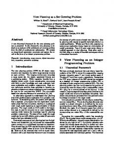
are probabilistic detection parameters to measure detection strength when a target point lies within the interval . It causes coverage value to exponentially decrease as the distance increase. All points that lie within a distance of from the sensor are said to be 1-covered. Beyond the distance , all the points have 0-coverage by this sensor (see Figure 1).
226
Attea & Hameed
Iraqi Journal of Science, 2014, Vol 55, No.1, pp:224-240
Figure 1 -Probabilistic sensing model.
To save energy, a subset of sensors from the sensor set should be activated into a duty-cycling sensor cover subset, to cover all the interested targets in . In the literature and under the traditional Boolean sensing model, the definition of the sensor cover could be formulated as: Definition 1: (Sensor Cover - SC). Given a WSN consists of target set and sensor set , where each sensor can be represented as a subset , such that if and only if . Any subset that can completely cover all the target set is termed as a sensor cover. However, considering probabilistic sensing model, the definition of the traditional sensor cover needs to be re-formulated, here, as: Definition 2 (Reliable Sensor Cover - RSC). Given a WSN consists of target set and sensor set , where each sensor can be represented as a subset , such that if and only if . Any subset that can satisfy a user coverage constraint to cover all the targets in is termed as a reliable sensor cover or reliable set cover. Formally speaking: (2) Now, the problem of finding the minimum number of sensors that reliably cover all the targets (here we called it minimum reliable set cover problem - MRSCP) can be formulated as: Definition 3 (Minimum Reliable Sensor Cover Problem - MRSCP). Given a collection of sensors, find the minimum number of sensors that reliably covers . Every cover is a subset of , , such that every element of belongs to at least one member of . A cover is said to contain a minimum number of sensors if for any other cover , . Formally speaking: (3) The proposed Genetic Algorithm The GA simulates the biological processes of natural selection, reproduction, and mutation to iteratively evolve species of individual solutions to become more and more adapted to the problem environment. The proposed GA can be described as a process formulated in the following formulafashion. Let , be the process that iteratively evolve a population of solutions, using genetic operators, toward the best set cover solution in terms of minimum number of sensors (i.e., sensor cost) that reliably cover all targets. Thus, the objective function of GA can be formulated for the minimum set cover problem as: (4) The best set cover solution will show up both active and sleep sensor sets. 3.1 Space and Solution Configurations The choice of a good solution representation is a critical issue for the applicability and performance of any evolutionary algorithm. Solution representation is highly problem dependent and related to the evolution operations. In our algorithm design, each individual solution of is represented as a fixed-length vector of size , where each controls the active/sleep scheduling of the corresponding sensor in . Thus,
(5)
227
Attea & Hameed
Iraqi Journal of Science, 2014, Vol 55, No.1, pp:224-240
Then, the whole configuration space for the GA can be created by the Cartesian product of activation/inactivation of all unassigned sensors: (6) where means inactive (i.e., unassigned) sensor, while means active (i.e., assigned) sensor. Let us to consider that handles only different individual solutions at a time. It starts with an initial random population and continues until a maximum number of generations has been reached. Each generation consists of four main operators: individual repair, parent selection, crossover, and mutation. Thus, can be decomposed into: (7) 3.2 Repair Operator and the Fitness Function Before evaluating each individual, infeasible set cover solutions should be transformed into feasible ones by means of a problem-specific repair operator. Infeasible solutions are those which suffer from either the existence of coverage-holes or let the targets to be over-covered by more than need sensors. The main idea of the proposed repair operator is to make hole-free targets coverage with as less number of sensors as possible. The process of the proposed repair operator is presented next (see Algorithm 1). (8) It takes as input the individual and the set of unassigned sensors . First, it check whether the active sensors set selected by (i.e., ) forms coverage-hole or dense-coverage under the user-specified reliability threshold . In case of coverage-hole, will randomly draw from set one sensor at a time and collect it with (i.e., and ) until the new set form hole-free set cover. On the other hand, if forms dense-coverage, will randomly deactivate one sensor at a time (i.e., and ) until it can form complete coverage with less number of sensors. Algorithm 1: Repair Operator ( , , 1: set to the active sensors selected by 2: 3: 4: 5: 6: 7: 8: 9: 10: 11: 12: 13: 14: 15:
if
)
/* no coverage hole */
while select a random sensor set set end while set /* now else /* coverage holes exist after sensors in */ while 0 select a random sensor set set end while end if
1 */ using the
Then, to evaluate each individual solution , the fitness function active sensors being selected by the corresponding solution. (9)
228
simply sums the number of
Attea & Hameed
Iraqi Journal of Science, 2014, Vol 55, No.1, pp:224-240
3.3 Selection, Crossover, and Mutation Operators The remaining genetic operators follow the de-facto standard operators found in the simple genetic algorithms. The binary tournament selection operator is used to choose one of two random individuals and . A proportion of pairs of parents are then selected for crossover. Two cut points , are randomly selected, and the participating parent individuals, are then swapped at . Each in the new individuals is then mutated with small probability . (10)
(11)
(12) The mechanisms of the genetic operators being defined by repair, fitness evaluation, selection, crossover and mutation transform a complete population of solutions into another complete population and after a specified number of generations , the best individual solution (in terms of minimum ) will be produced. The definition of the best individual can be formulated as: (13) 3.4 Post-heuristic Operator The best solution provided by the can further be improved in terms of coverage reliability by forwarding it to a post-heuristic operator dedicated for this purpose. Algorithm 2 presents the steps of this heuristic. It operates by exploiting the existing unassigned sensors (being gathered in ) and/or replacing the existing active sensors (being gathered in ). Algorithm 2: Post-Heuristic ( ) 1: /* a new cover will be formed */ set 2: set to the sensors from both and 3: 4: 5: 6: 7: 8: 9: 10: 11:
set contributed sensors set set while select a sensor that contributes to the most reliable coverage to a target set ; end while remove remove
4 Performance Evaluations In this section we will measure the performance of the proposed GA for solving MSCP in WSNs. The evaluation is presented in terms of number of active sensors obtained (i.e., sensors cost), and coverage reliability. The results are obtained after setting WSNs and algorithm parameters into the following. The simulation area is square-shaped with side length . The simulation is divided according to:
229
Attea & Hameed
Iraqi Journal of Science, 2014, Vol 55, No.1, pp:224-240
1. Five different settings for the number of targets
.
2. Three different settings of sensor density:
. 3. For each test instance group composed from 1 and 2, we will vary the sensing range of the sensor nodes to eight different values . Thus, we have a total of different test instances (composed from 1, 2 and 3). Each test instance includes 10 random WSNs with different configurations. Thus the overall simulation examines a total of random networks. Uncertainty level is set to units, both and are set to , and is set to . The setting of the probabilistic coverage parameters also influences the overall network's coverage reliability. As studying the impact of varying these parameters is out of the scope of this paper, we fixed these parameters to one setting. Population size is set to and will be allowed to evolve times. 4.1 Impact of WSN's and Parameters on Solution Quality First, figures 2-6 depict the sensors cost percentage while varying number of targets and sensing range for the three different settings of sensor density. is defined as the ratio between the number of active sensors used in the generated best individual solution and the total number of sensor nodes , i.e.,: (14) For further qualitative presentation, figures 6 and 7 depicts for the three different settings of sensor density, i.e., and and the eight settings of sensing range, while fixing target size to its extreme values, i.e., and . Figures 9 – 11 qualitatively depict the whole performance of the proposed GA for WSNs, where results are projected in 3D space. Number of Targets = 10 8
7
Sensor C ost%
6
5
4
3
2
1
0
100
125
150
Sensor Density for Rs = 100, 200,..., 800
Figure 2- Percentage of sensors cost for and
WSNs, where .
Number of Targets = 20 15
Sensors Cost%
10
5
0
100
125
150
Sensor Density for Rs = 100, 200,..., 800
230
,
Attea & Hameed
Iraqi Journal of Science, 2014, Vol 55, No.1, pp:224-240
Figure 3- Percentage of sensors cost for and
WSNs, where .
,
WSNs, where .
,
WSNs, where .
,
WSNs, where .
,
Number of Targets = 30 18 16 14
Sensors Cost%
12 10 8 6 4 2 0
100
125
150
Sensor Density for Rs = 100, 200,..., 800
Figure 4- Percentage of sensors cost for and Number of Targets = 40 25
Sensors Cost%
20
15
10
5
0
100
125
150
Sensor Density for Rs = 100, 200,..., 800
Figure 5-Percentage of sensors cost for and Number of Targets = 50 25
Sensors Cost%
20
15
10
5
0
100
125
150
Sensor Density for Rs = 100, 200,..., 800
Figure 6- Percentage of sensors cost for and
231
Attea & Hameed
Iraqi Journal of Science, 2014, Vol 55, No.1, pp:224-240
Number of Targets = 10 8 m = 100 m = 125 m = 150
7
6
Sensors Cost%
5
4
3
2
1
0 100
200
300
400
500
600
700
800
Sensing Range (Rs)
Figure 7- Percentage of sensors cost for and
WSNs, where .
,
Number of Targets = 50 25 m = 100 m = 125 m = 150
Sensors Cost%
20
15
10
5
0 100
200
300
400
500
600
700
800
Sensing Range (Rs)
Figure 8- Percentage of sensors cost for and
WSNs, where .
,
Sensor Density = 100
25
Sensors Cost%
20 15 10 5 0 50 40 30 20
Number of Targets
10
100
200
300
400
500
600
700
800
Sensing Range (Rs)
Figure 9- 3D projection of results. Coordinate ( : sensing range, simulation is experimented under networks with
232
: number of targets, : SC%). The 100.
Attea & Hameed
Iraqi Journal of Science, 2014, Vol 55, No.1, pp:224-240
Sensor Density = 125
20
Sensors Cost%
15
10
5
0 50 40 30 20 10
Number of Targets
100
200
300
400
500
600
700
800
Sensing Range (Rs)
Figure 10- 3D projection of results. Coordinate ( : sensing range, simulation is experimented under networks with
: number of targets, : SC%). The 125.
Sensor Density = 150
20
Sensors Cost%
15
10
5
0 50 40 30 20
Number of Targets
10
100
200
300
400
500
600
700
800
Sensing Range (Rs)
Figure 11- 3D projection of results. Coordinate ( : sensing range, simulation is experimented under networks with
: number of targets, : SC%). The 150.
Results in the previous figures reveal that the proposed GA can effectively find a minimum number of active sensors from the whole sensors set, and thus configuring an energy-efficient WSN. The characteristic components of the proposed GA (being specified mainly by the chromosome binary representation and the proposed repair operator) is found to be very suitable for solving MRSCP. As expected from the qualitative results depicted in figures 7 - 10, increasing sensor density and/or sensing range provides algorithms with more alternatives for constructing complete and reliable set cover with minimum number of active sensors. On the other hand, increasing target size lets the algorithm to consume more sensors. 4.2 At Any-Time Performance of GA Figures 12-14 depicts the any-time performance of the proposed GA while fixing target size and sensor density to their extremes, 50 and 150, respectively and varying sensing range to three different values, .
233
Attea & Hameed
Iraqi Journal of Science, 2014, Vol 55, No.1, pp:224-240
Number of Targets = 50; Sensor Density = 150; Rs = 100 400 380 360
Sensors Cost
340 320 300 280 260 240 220
0
50
100
150
200
250
300
350
400
450
500
Generation Number
Figure
12
Any-time
evolution
of
,
sensors and
cost
sensors and
cost
sensors and
cost
for
WSNs,
where
for
WSNs,
where
for
WSNs,
where
.
Number of Targets = 50; Sensor Density = 150; Rs = 200 90
85
Sensors Cost
80
75
70
65
60
55
0
50
100
150
200
250
300
350
400
450
500
Generation Number
Figure
13
Any-time
evolution
of
,
.
Number of Targets = 50; Sensor Density = 150; Rs = 300 70
65
Sensors Cost
60
55
50
45
40
0
50
100
150
200
250
300
350
400
450
500
Generation Number
Figure
14-
Any-time
evolution ,
of
.
The results in figures 11-13 show up that sensing radius increases, the convergence time towards the minimum number of sensors is also increased. When , we can see that the convergence occurs after 65 generations. Increasing to , helps the algorithm to converge to the required solution after generations. Moreover, letting , further increases the convergence time to less than generations. 4.3 Impact of Post-heuristic Operator The performance of the proposed GA is presented, here, before and after performing the postheuristic operator. Figures 15 –22 depict coverage reliability and sensors cost percentage being resulted from the proposed GA before and after applying post-heuristic. As we stated before that probabilistic coverage parameters are fixed throughout all simulations, we evaluate, as reference values, the average coverage reliability (i.e., the average signal strength being detected from all the targets) of all network configurations in each test instance.
234
Attea & Hameed
Iraqi Journal of Science, 2014, Vol 55, No.1, pp:224-240
Number of Targets = 10
Coverage Reliability before heuristic operator
0.7
0.6
0.5
0.4
0.3
0.2
0.1
0
100
125
150
Sensor Density for Rs = 100, 200,..., 800
Figure
15-
Coverage
reliability
before
applying
,
heuristic operator and
for
heuristic operator and
for
WSNs: }.
Number of Targets = 10
Coverage Reliability after heuristic operator
1 0.9 0.8 0.7 0.6 0.5 0.4 0.3 0.2 0.1 0
100
125
150
Sensor Density for Rs = 100, 200,..., 800
Figure
16-
Coverage
reliability
after
applying
,
WSNs: }.
Number of Targets = 10 8
Sensor Cost before heuristic operator
7
6
5
4
3
2
1
0
100
125
150
Sensor Density for Rs = 100, 200,..., 800
Figure
17-
Sensor
cost
before ,
applying
235
heuristic
operator and
for
WSNs: }.
Attea & Hameed
Iraqi Journal of Science, 2014, Vol 55, No.1, pp:224-240
Number of Targets = 10 10 9
Sensor Cost after heuristic operator
8 7 6 5 4 3 2 1 0
100
125
150
Sensor Density for Rs = 100, 200,..., 800
Figure
18-
Sensor
cost
after ,
applying
heuristic
operator and
for
WSNs: }.
Number of Targets = 50
Coverage reliability before heuristic operator
0.8
0.7
0.6
0.5
0.4
0.3
0.2
0.1
0
100
125
150
Sensor Density for Rs = 100, 200,..., 800
Figure
19-
Coverage
reliability
before
applying
,
heuristic operator and
for
heuristic operator and
for
WSNs: }.
Number of Targets = 50
Coverage Reliability after heuristic operator
1 0.9 0.8 0.7 0.6 0.5 0.4 0.3 0.2 0.1 0
100
125
150
Sensor Density for Rs = 100, 200,..., 800
Figure
20-
Coverage
reliability
after
applying
,
236
WSNs: }.
Attea & Hameed
Iraqi Journal of Science, 2014, Vol 55, No.1, pp:224-240
Number of Targets = 50
Sensor Cost before heuristic operator
25
20
15
10
5
0
100
125
150
Sensor Density for Rs = 100, 200,..., 800
Figure
21-
Sensor
cost
before ,
applying
heuristic
operator and
for
operator and
for
WSNs: }.
Number of Targets = 50 40
Sensor Cost after heuristic operator
35
30
25
20
15
10
5
0
100
125
150
Sensor Density for Rs = 100, 200,..., 800
Figure
22-
Sensor
cost
after ,
applying
heuristic
WSNs: }.
We can see that the proposed post-heuristic operator can exploit the existence of the redundant sensors to improve its covers reliability. In almost all of the test instances, the proposed post-heuristic operator attains reliable coverage of while consuming very few extra sensors. For example, in figures 16 and 20, we see that the coverage reliability reaches its full certainty when . Also, for , the post-heuristic operator achieves high coverage reliability with more than . Tables 1 and 2 quantitatively present the results of figures 16 and 20, respectively. The positive impact of the proposed post-heuristic operator can be returned back to its ability to select those sensors which lie near the targets such that their distances from the targets do not exceed . However, when lessening sensor density and/or sensing range to their low extremes (i.e., and ), the chance of finding sensors nearby targets or finding sensing areas that cover targets also decreases. The results also demonstrate that there should be a tradeoff between the two contradictory criteria of getting minimum number of active sensors and high covers reliability.
237
Attea & Hameed
Iraqi Journal of Science, 2014, Vol 55, No.1, pp:224-240
Table 1-Comparison of coverage reliability and sensors cost before and after applying post-heuristic operator. Results are presented for 24 test instances ( 0) for WSNs in each test instance with , and . Before post-heuristic After post-heuristic operator operator Coverage Coverage reliability reliability 0.1628 0.1350 7.9 0.6037 9.5 0.1688 0.1297 3.2 0.9834 9.1 0.2539 0.2333 2.5 1.0 8.4 0.3317 0.4379 2.3 1.0 7.2 0.4102 0.4042 2.0 1.0 5.8 0.4794 0.5429 1.8 1.0 5.5 0.5396 0.4957 1.4 1.0 4.6 0.5917 0.5812 1.0 1.0 4.4 0.1539 0.1355 6.64 0.6051 7.76 0.1590 0.0807 2.64 0.9633 7.6 0.2510 0.2635 2.24 1.0 6.96 1.0 0.3374 0.3139 1.84 6.16 1.0 0.4199 0.4509 1.60 5.12 1.0 0.4816 0.4802 1.36 4.24 1.0 0.5358 0.6045 1.28 4.08 1.0 0.5863 0.5845 1.04 3.36 0.1582 0.2046 5.1333 0.7415 6.3333 0.1721 0.1513 2.2667 0.9908 5.9333 0.2687 0.1974 1.8667 1.0 5.3333 1.0 0.3532 0.3836 1.6000 4.8667 1.0 0.4163 0.4211 1.3333 4.2 1.0 0.4705 0.4636 1.1333 3.7333 1.0 0.5244 0.5048 0.8667 3.3333 1.0 0.5742 0.5800 0.7333 2.7333 Table 2- Comparison of coverage reliability and sensors cost before and after applying post-heuristic operator. Results are presented for 24 test instances ( ) for WSNs in each test instance with , and . Before post-heuristic After post-heuristic operator operator Coverage Coverage reliability reliability 0.1741 0.2496 23.2 0.6024 37.0 0.1682 0.2155 5.9 0.9612 32.6 0.2577 0.3099 4.1 0.9981 23.5 0.3447 0.4261 3.7 1.0 16.3 0.4226 0.5081 3.0 1.0 12.1 0.4869 0.6659 2.8 1.0 9.4 0.5384 0.6769 2.0 1.0 7.5 0.5832 0.7201 2.0 1.0 6.5 0.1722 0.2613 17.76 0.6957 30.0 0.1685 0.2084 4.48 0.9774 24.24 0.2595 0.3213 3.28 1.0 17.68 1.0 0.3472 0.4244 2.88 13.44 1.0 0.4261 0.5317 2.4 10.0 1.0 0.4887 0.6124 2.08 7.36 1.0 0.5437 0.6383 1.6 6.96 1.0 0.5862 0.7017 1.44 5.52
238
Attea & Hameed
Iraqi Journal of Science, 2014, Vol 55, No.1, pp:224-240 0.1717 0.1765 0.2660 0.3466 0.4130 0.4713 0.5255 0.5743
0.2442 0.2086 0.2869 0.4144 0.5240 0.6550 0.6047 0.7189
15.6 3.9333 2.9333 2.5333 2.1333 1.9333 1.3333 1.3333
0.7467 0.9942 1.0 1.0 1.0 1.0 1.0 1.0
26.5333 21.2 14.6667 10.9333 8.2 6.4 5.4667 4.9333
Also from the tables, one can see that the collaboration between the proposed GA and post-heuristic operator consumes very few sensors from the whole sensor set (in the worst case no more than in test instance ) to achieve reliable coverage higher than the average reliability . 4.4 Worst Case Time Complexity Here we will compute the worst-case computational complexity of the proposed GA for solving minimum reliable set cover problem (MRSCP). Without loss of generality, the computational complexity of any single-objective genetic algorithms is where is the size of solutions to be evolved, via certain evolution operators, for iterations. Now, let us consider the computation time needed for the most critical parts of the proposed algorithm when applied for solving MRSCP. The most critical part which represents the computation time bottleneck in the proposed GA is the proposed repair operator (Algorithm 1) which costs the most computation time and in the worst-case time it linearly related to the maximum number of sensors and targets . Thus, the worst-case time complexity of the proposed GA can formally be described as: (15) 5 Conclusions In this paper, we have addressed designing energy-efficient WSNs with reliable coverage of the target area. The problem is modeled a minimum reliable set cover problem (MRSCP), which introduce the concept of probabilistic coverage as a more realistic coverage model for constructing the set cover. A genetic algorithm is proposed to construct a reliable set cover, where the total number of sensors used in the set is to be minimized. The result of the GA is then forwarded to a post-heuristic operator to improve the coverage reliability of the set cover. The performance of the proposed genetic algorithm is investigated in this paper under different simulation setting. The results of the simulations reveal that the number of active sensors used in the constructed set cover affected by the WSN design parameters including target size, sensor density, and sensor range. The results of this paper currently motivate us to investigate the possibility of applying multi-objective evolutionary algorithms (like MOEA/D, NSGA-II, and MOPSO [21]-[24]) to the combined optimization problem of both minimum set cover problem and cover reliability problem and handling both objective functions simultaneously instead of applying consecutive optimization mechanisms. Also, as a scope of further work, another quality of service (QoS) merit could be used to constraint the defined MRSCP. For example, different targets may need different priority of sensing quality and thus the optimization problem should reflect this diversified QoS coverage constraint in its formulation. References 1. Garey M. R. and Johnson D. S. 1979, Computers and Intractability. A Guide to the Theory of NPCompleteness. Freeman, New York. 2. Slijepcevic S. and Potkonjak M. 2001, Power efficient organization of wireless sensor networks, in Proceeding. IEEE Int. Conference Commun, (2), pp: 472–476. 3. Cardei M., Thai M., Li Y., and Wu W. 2005, Energy-Efficient Target Coverage in Wireless Sensor Networks, IEEE INFOCOM, pp: 1976-1984. 4. Tian D. and Georganas N. D. 2002, A coverage-preserving node scheduling scheme for large wireless sensor networks, in Proceeding. 1st Assoc. Comput. Machinery Int. Workshop Wireless Sensor Netw. Appl, pp: 32–41. 5. Wang X., Xing G., Zhang Y., Lu C., Pless R., and Gill C. 2003, Integrated coverage and connectivity configuration in wireless sensor networks, in Proceeding. 1st Int. Conference. Embedded Netw. Sensor Syst., Los Angeles, CA, pp: 28–39.
239
Attea & Hameed
Iraqi Journal of Science, 2014, Vol 55, No.1, pp:224-240
6. Liu Y. and Liang W. 2005, Approximate coverage in wireless sensor networks,” in Proceeding. IEEE Conference. Local Comput. Netw, pp: 68–75. 7. Gupta H., Zhou Z., Das S. R., and Gu Q. 2006, Connected sensor cover: Self-organization of sensor networks for efficient query execution, IEEE/Assoc. Comput. Machinery Trans. Netw., 14(1), pp:55-67. 8. Ai J. and Abouzeid A. A. 2006, Coverage by directional sensors in randomly deployed wireless sensor networks, J. Comb. Optim., 11(1), pp: 21–41. 9. Funke S., Kesselman A., Kuhn F., Lotker Z., and Segal M. 2007., Improved approximation algorithms for connected sensor cover, Wireless Netw., 13(2), pp: 153–164. 10. Zhou Z., Das S. R., and Gupta H. 2009, Variable radii connected sensor cover in sensor networks,Assoc. Comput. Machinery Trans. Sensor Netw., 5(1), article 8, pp: 1–36. 11. Martins F. V. C., Carrano E. G., Wanner E. F., Takahashi R. H. C., and Mateus G. R. 2009, A dynamic multiobjective hybrid approach for designing wireless sensor networks, IEEE Congr. Evol. Comput, pp: 1145–1152. 12. Cardei M. and Du D.-Z. 2005, Improving wireless sensor network lifetime through power aware organization, Wireless Netw., 1193), pp: 333–340. 13. Cardei I. and Cardei M. 2008, Energy-Efficient Connected-Coverage in Wireless Sensor Networks, International Journal on Sensor Networks, 3. 14. He J. , Xiong N. , Xiao Y. and Pan Y. 2010, A Reliable Energy Efficient Algorithm for Target Coverage inWireless Sensor Networks, in:·Proceeding ICDCSW '10 Proceedings of the IEEE 30th International Conference on Distributed Computing Systems Workshops, pp: 180-188. 15. Lai C., Ting C., and Ko R. 2007, An Effective Genetic Algorithm to Improve Wireless Sensor Network Lifetime for Large-Scale Surveillance Applications, IEEE Congr. Evol. Comput, pp: 3531–3538. 16. Hu X. , Zhang J. , Yu Y. , Chung H. S. , Li Y. , Shi Y. , Luo X. 2010, Hybrid Genetic Algorithm Using a Forward Encoding Scheme for Lifetime Maximization of Wireless Sensor Networks, IEEE Trans. Evol. Comp., 14(5), pp: 766-781. 17. Gil J.M., and Han Y.H. 2011, A Target Coverage Scheduling Scheme Based on Genetic Algorithms in Directional Sensor Networks, Sensors, 11(2), 1888-1906; 18. Elfes A. 1987, Sonar-based real-world mapping and navigation, IEEE Journal of Robotics and Automation, 3(3), pp: 249–265. 19. Ghosh A. and Das S. K. 2006, Coverage and Connectivity Issues in Wireless Sensor Networks, Chap. 6, Mobile, Wireless, and Sensor Networks: Technology, Applications, and Future Directions, R. Shorey, A. L. Ananda, M. C. Chan, and W. T., John Wiley & Sons, Inc. 20. Hossain A., Biswas P. K., Chakrabarti S. 2008, Sensing Models and its Impact on Network Coverage in Wireless Sensor Network, In the Proceedings of 3rd International Conference on Industrial and Information Systems(ICIIS 2008), IIT Kharagpur., India. 21. Huang C.F. and Tseng Y.C. 2005, The coverage problem in a wireless sensor network, Mobile Netw. Appl., 10(4), pp: 519–528. 22. Deb K. 2002, Multi-Objective Optimization using Evolutionary Algorithms. Wiley, Chichester, 2001. 23. C.A. Coello Coello, D.A. Van Veldhuizen, and G.B. Lamont, Evolutionary Algorithms for Solving Multi-Objective Problems. Kluwer, New York. 24. Zhang Q. and Li H. 2007, MOEA/D: A multi-objective evolutionary algorithm based on decomposition, IEEE Transactions on Evolutionary Computation, 11(6), pp: 712–731,. 25. Coello C. A., Toscano-Pulido G., Salazar-Lechunga M. 2004., Handling multiple objectives with particle swarm optimization, IEEE Trans on Evol Comput, 8(3), pp:256–279,.
240