A genetic algorithm for vehicle routing with backhauling - Springer Link

@ 1996 Kluwer

A Genetic Algorithm

Academic

Applied Intelligence Publishers. Manufactured

6, 345-355 (1996) in The Netherlands.

for Vehicle Routing with Backhauling

JEAN-YVES POTVIN Centre de recherche sur les transports, Universite’ de Montreal, C.P. 6128, Succ. Centre-Ville, Montreal (Quebec), Canada H3C 357; and Departement d’informatique et de recherche operationnelle, Universite’ de Montreal, C.P. 6128, Succ. Centre-Ville, Montreal (Quebec), Canada H3C 3J7

Laboratoire d’lnformatique

CHRISTOPHE DUHAMEL et de Mode’lisation des Systemes, ISIMA, B.l? 12.5, 63173 Aubiere Cedex, France

FRANCOIS GUERTIN Centre de recherche sur les transports, Universite’ de Montreal, C.l? 6128, Succ. Centre-Ville, Montreal (Quebec), Canada H3C 3J7

Abstract. In this paper, a greedy route construction heuristic for a vehicle routing problem with backhauling is described. This heuristic inserts customers one by one into the routes using a fixed a priori ordering of customers. Then, a genetic algorithm is used to identify an ordering that produces good routes. Numerical comparisons are provided with an exact algorithm and with other heuristic approaches. Keywords:

1.

vehicle routing, backhauling, time windows, genetic algorithms, heuristics

Introduction

The Vehicle Routing Problem with Backhauls (VRPB) can be stated as follows: given a central depot, a fleet of vehicles and a set of customers with known demands for service (e.g., a quantity of goods to be picked up or delivered), find a set of routes, originating and ending at the depot, that services all customers at minimum cost. In this problem, each vehicle services both delivery points (linehaul customers) and pick-up points (backhaul customers). In the grocery industry, for example, the linehaul and backhaul customers could be supermarkets and grocery suppliers, respectively. In many applications, the pick-ups must be done after the deliveries in each route. This constraint arises in practice because it is often inconvenient to rearrange delivery loads on-board in order to accommodate new pick-up loads, and deliveries are usually higher-priority stops than pick-ups. Due to the finite capacity of each vehicle, the routes must also satisfy capacity constraints. That

is, the load should never exceed the capacity of the vehicle. In this paper, we consider a variant of this problem where each customer must also be serviced within a specified time interval (or time window). In particular, a vehicle cannot arrive at a customer location after its time window’s upper bound. However, the vehicle can arrive at a customer location before the lower bound. In this case, a waiting time is incurred. The objective is to minimize the total distance traveled, while satisfying all constraints. When all customers are pick-up points (or delivery points), the VRPBTW reduces to the vehicle routing problem with time windows or VRPTW. Alternatively, when the time windows are arbitrarily large, the VRPBTW reduces to the vehicle routing problem with backhauls or VRPB. Since the VRPB and the VRPTW are NP-complete, this is also the case for the VRPBTW. Although different heuristic and exact problemsolving approaches may be found in the literature for

346

Potvin, Duhamel and Guertin

both the VRPB [4, 7, 1 l] and the VRPTW [8, 12, 15, 17-191, only one algorithm is reported for the variant of the VRPB with time window constraints [lo]. In this work, a column generation technique is used to solve a set partitioning formulation of the problem. This algorithm found optimal solutions to different test problems with up to 100 customers. Problem-solving approaches for vehicle routing problems can be divided into three broad classes: route construction heuristics that “build” routes through the insertion of new customers, route improvement heuristics that modify the location of customers within existing routes through exchange procedures, and composite heuristics that combine both route construction and route improvement procedures. In this paper, a route construction heuristic for the VRPBTW is proposed. This heuristic inserts the customers one by one into the routes based on a fixed a priori ordering of customers. Using this ordering, each customer is inserted at the location that minimizes a weighted sum of detour and service delay in the route. This is a “greedy” heuristic because the best insertion place for each unrouted customer is chosen at each iteration. It is also “myopic” because the insertion of each customer is performed without any consideration for the remaining unrouted customers. A distinctive feature of our approach is the use of a genetic algorithm to search for the best ordering of customers during the insertion procedure. This hybrid problem-solving approach has already been proposed for other combinatorial optimization problems with side constraints [3, 6, 161. Under this scheme, the genetic algorithm does not explicitly consider the side constraints, because they are satisfied through the construction of the solution by the insertion heuristic. Accordingly, the genetic algorithm only searches for a good ordering of customers. This paper describes a similar problem-solving approach for the VRPBTW. Section 2 first introduces our greedy insertion heuristic. Then, the evolution paradigm is briefly introduced in Section 3. In Section 4, our genetic algorithm is described. Finally, computational results on a set of test problems are reported. 2.

The Insertion

route is created with the first customer in this ordering. Therefore, the initial route only services a single customer (i.e., the vehicle leaves the depot, services the customer and comes back to the depot). Then, the next customer in the ordering is considered, and the feasible insertion place that minimizes a weighted sum of detour and service delay in the route is chosen (using the weights suggested in [17]). If no feasible insertion place is found, a new route is created to service this customer. This procedure is repeated for all customers in the ordering. It is worth noting that feasible insertion places over all available routes are looked for, before a new route is created for a customer. For example, if five customers are to be serviced, and the ordering is 1, 2, 3, 4, 5, customer 1 is used to create the first route. Then, customer 2 is inserted in this route, followed by customer 3. At this point, we assume that there is no feasible insertion place for customer 4. Consequently, a second route is created to service customer 4. Then customer 5 can be inserted either in the first or second route, depending on the location of its best feasible insertion place. Obviously, different solutions can be produced by modifying the insertion order of the customers. The method uses an insertion cost measure ci to guide the insertion of the next customer in the ordering. Namely, the best insertion place for customer u minimizes the cost cl over all feasible insertion places between two consecutive customers i and j in the routes, where: cl(i,

u, j)

=

cf~ x

cll(i,

(Y1+a2=

u, 1,

j>

+ a1

(~2 x >

c12(i,

0, a2

2

u,

j),

0,

cll(i, u, j> = 4, + duj - CLx dij, cn(i, u, j> = b,i - bj, dij is the distance (in time units) between i and j. bj is the current service time at customer j. b,j is the new service time at customer j due to the insertion of customer u before j. opt is the weight for the detour. CQ is the weight for the service delay at customer j. p is the weight for the distance between customers i and j in ci 1.

Heuristic

Our greedy insertion heuristic is derived from Solomon’s work [ 171, and can be described as follows. Given some a priori ordering of customers, the first

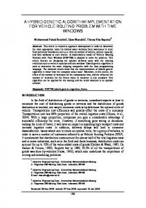
Note that the insertion cost cl of customer u is a weighted sum of two components: ct 1, the detour (in time units) and ~12,the service delay at customer j due to the insertion of customer u (see Fig. 1).

A Genetic Algorithm for Vehicle Routing with Backhauling

u

347

can be used to find the best possible ordering. In Section 3, a simple genetic algorithm is briefly introduced. Then, a specific implementation for our ordering problem is described.

3.

A Simple

Genetic

Algorithm

In order to apply a genetic algorithm to a given problem, solutions to this problem must first be encoded as chromosomes (typically, bit strings). Then, an evaluation function that returns the fitness or quality of each chromosome is defined. Using these two components, a simple genetic algorithm can be summarized as follows: Fi,qure

I

An insertion

place for customer

u in a route.

In order to be feasible, the insertion of the new customer must satisfy the capacity and time window constraints. Moreever, the backhaul customers must always follow the linehaul customers in each route. The latter constraint implies that a linehaul customer can only be inserted at the following locations:

(4 Between the depot and the first linehaul customer, (b) Between two linehaul customers, (cl Between the last linehaul customer and the first backhaul customer,

(4 Between the last linehaul customer and the depot, if there is no backhaul customer. Obviously, equivalent constraints apply to the insertion of a backhaul customer. In [3], a equivalent insertion heuristic is described. However, the routes are all created at once, rather than one by one. That is, many routes are created with the first customers in the ordering, and the remaining unrouted customers are inserted into any one of those routes. Since the number of routes that must be constructed to service all customers is not known in advance, many different runs must be performed with an increasing number of routes until a feasible solution is found. This difficulty does not arise with our sequential approach, because the routes are created one by one, as needed, until all customers are serviced. Since the insertion heuristic uses a fixed ordering of customers to construct the routes, a genetic algorithm

Step I (Initialization). Create an initial random population of chromosomes and evaluate each chromosome. Set the current population to this initial population. Step 2 (Reproduction). Select two parent chromosomes from the current population. The selection process is stochastic and a chromosome with high fitness is more likely to be selected. Step 3 (Recombination). Generate two offspring from the two parent chromosomes by exchanging bit strings (crossover). Step 4 (Mutation). Apply a random mutation to each offspring (with a small probability). Step 5. Repeat Steps 2, 3 and 4, until the number of offspring in the new population is the same as the number of chromosomes in the old population. Step 6. Evaluate each offspring. Set the current population to the new population of chromosomes and go back to Step 2. This procedure is repeated for a fixed number of generations, or until no more improvement is observed. The best chromosome generated during the search is the final result of the genetic algorithm. Through this process, it is expected that an initial population of randomly generated chromosomes with low fitness values will improve as parents are replaced by better offspring. In the following, the main components of the genetic search are briefly described. First, the encoding transforms a solution to a problem into a bit string. For example, if the problem is to maximize a numerical function f whose domain is a set of integers, then each

348

Figure

Pohk, Duhamel and Guertin

2.

0 1

010 11 1

0 1

0 1 One-point

0 1

0 1

(parent 1) (parent 2)

0

0

(offspring 1) (offspring 2)

111 0

crossover

on two bit strings

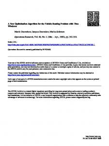
chromosome can represent an integer in base-2 notation. In this case, the fitness of each chromosome is f(x), where x is the integer encoded in the chromosome. The reproduction phase favors the best chromosomes through a bias in the selection process. Namely, chromosomes with high fitness are more likely to be selected as parents. Once the parents have been selected, the recombination phase creates two new offspring through the exchange of bit strings taken from two parent chromosomes. Here, the underlying assumption is that a better chromosome can be produced by combining bit patterns taken from two good chromosomes. An example of a one-point crossover is shown in Fig. 2 for two parent bit strings of length 5. Here, the cross point is (randomly) chosen between the second and third bit. As we can see, the end parts of both parents are swapped to create two offspring. Finally, the mutation phase is aimed at maintaining a minimum level of diversity in the population via random modifications to the bit values. Namely, the mutation operator flips bit values from 0 to 1 or from 1 to 0 with a small probability at each position of each offspring. A good level of diversity in the population is crucial to the effectiveness of the search. If the population is composed of similar chromosomes, the search will not make any progress because the offspring will look like their parents. In the next section, an adaptation of this simple genetic algorithm for our ordering problem is described. 4.

The Ordering

Problem

Here, the genetic algorithm must find a good ordering of customers for the route construction heuristic. Accordingly, our implementation departs from the classical scheme in two important ways: (a) chromosomes are sequences of integers rather than sequences of bits (where each integer represents a particular customer).

(b) Specialized crossover and mutation operators are designed to produce new orderings (or permutations) from old ones. Given these particularities, the main components of our genetic algorithm will now be introduced. 4.1.

Representation

As mentioned before, an ordering is encoded as a sequence of integers. Assuming that five customers must be serviced, the ordering 1 2 3 4 5 means that customer 1 will be the first to be inserted in a route, followed by customer 2, etc. 4.2.

Reproduction

The fitness of each chromosome is derived from the quality of the solution produced by the insertion heuristic, using the ordering encoded on the chromosome. In this application, solution quality is based on total distance, as in [3, lo]. The rank of each chromosome in the population is used to evaluate its fitness [ 1, 201. In the example below, the population is composed of three chromosomes, encoding three different orderings. The value of the solution produced by the insertion heuristic is shown on the same line. In this example, chromosome 2 gets rank 1 because this ordering has produced the minimum distance, while chromosomes 1 and 3 get ranks 2 and 3, respectively. Chromosome

Distance

Rank

12345

1612.0

2

32415

1560.0

1

1680.0

3

2435

1

With these ranks, the fitness of a chromosome of rank i is computed as follows: fitnessi = Max - [(Max - Min) x (i - l)/(n

- l)],

where n is the number of chromosomes in the population. Hence, the best ranked chromosome gets fitness value Max and the worst chromosome gets fitness value Min. In the current implementation, Max and Min are set to 1.2 and 0.8, respectively. Then, a fitness proportional selection scheme is applied to these values. Namely, the selection probability

A Genetic Algorithm for Vehicle Routing with Backhauling

for a chromosome of rank i is: fittleSSi Pi

=

&=,

fitneSSi

,,,,, n fitlleSSj

=

7

It is worth noting that the summation over all fitness values in a population of size n is equal to n, because Min + Max = 2 and the average fitness is 1. Since n different selections (with replacement) must be performed in order to select n parents and generate n offspring, the expected number of selections Ei for a chromosome of rank i is: Ej = n

X

pj = fitnessj.

Hence, the fitness of each chromosome is also equal to its expected number of selections. For example, the best chromosome with fitness Max = 1.2, is expected to be selected 1.2 times on average over n different trials, while the worst chromosome is expected to be selected 0.8 times on average. As we can see, the gap between the best and the worst chromosome is not very large. Accordingly, the selection process is just slightly biased toward the best chromosomes. This is a way to favor the exploration of new regions of the search space. Exploration can be favored during the selection phase, due to a conservative generation replacement scheme (see Section 4.5). In order to reduce the variance associated with pure proportional selection (where each chromosome can be selected between 0 and n times over n different trials), stochastic universal selection or SUS is applied to the fitness values. This approach guarantees that the number of selections for any given chromosome is at least the floor, and at most the ceiling, of its expected number of selections [2]. 4.3.

Recombination

The permutation operator introduced in this section is an intermediate approach between “general purpose” permutation operators like OX [5, 131, and the heuristically-biased MXl and MX2 operators [3]. In the first case, the crossover operator generates new permutations through manipulations that do not exploit any heuristic information about the problem. Conversely, the MXI and MX2 operators exploit the precedence relationship established among the customers in regard to their time windows.

349

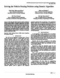
For example, the MXl operator works as follows. Starting at position 1, the customers on the two parent chromosomes are compared, and the customer with the earliest time window is introduced in the offspring. Then, the procedure is repeated at the next position, until all positions are done. In Fig. 3, we assume that the precedence relationship among the customers in regard to the time windows is 1, 2, 3, 4, 5. Starting at position 1, customers 1 and 4 are compared. Since the time window at customer 1 occurs before the time window at customer 4, customer 1 is introduced in the offspring (Fig. 3(a)). Now, in order to produce a valid ordering, customers 1 and 4 are swapped on parent 2. Then, customers 3 and 5 are compared at position 2, and customer 3 is introduced in the offspring (Fig. 3(b)). Customers 5 and 3 are swapped on parent 1, etc. The resulting offspring is shown in Fig. 3(e). The crossover operator MX2 works in a similar way (a complete description may be found in [3]). Note that both operators are strongly biased in favor of customers

(a) parent 1 parent 2

: :

1 4

5 3

2 1

3 2

4 5

offspring

:

1

-

-

-

-

parent 1 parent 2

: :

1 1

5 i!

2 4

3 2

4 5

offspring

:

1

3

-

-

-

parent 1 parent2

: :

1 1

3 3

2 4

5 2

4 5

offspring

:

1

3

2

-

-

parent 1 parent 2

: :

1 1

3 3

2 2

3 4

4 5

offspring

:

1

3

2

4

-

parent 1 parent 2

: :

1 1

3 3

2 2

4 4

5 5

offspring

:

1

3

2

4

5

(b)

Cc)

(4

(4

Figure

3.

MXl

crossover.

350

Potvin, Duhamel and Guertin

with early time windows. This bias is likely to lead to offspring that do not depart much from the precedence relationship established among the customers in regard to their time windows (i.e., 1, 2, 3,4,5). In order to prevent premature convergence, a new operator which is not as strongly biased as the MX operators was devised. This operator, called 1X, is similar to the classical one-point crossover. Accordingly, a cross point is randomly chosen on both chromosomes, and the end parts are exchanged to create two new offspring. In the process, some customers are duplicated on each offspring, while other customers are left apart. The duplicates are eliminated, and the customers that are missing take the available positions. When many customers are left apart, the customer with the earliest time window is inserted at the first available position, the customer with the second earliest time window is inserted at the second available position, etc. In Fig. 4, a cross point is randomly chosen between the second and third position on each parent chromosome. Then, the end parts are exchanged to create two new offspring (in the figure, only one offspring is shown). In the process, customers 1 and 5 are duplicated on the offspring and customers 3 and 4 are left apart. Hence, customers 1 and 5 are removed and replaced by customers 3 and 4, respectively. Note that customer 3 is inserted at the first available position, assuming that the precedence relationship among the customers in regard to the time windows is 1, 2, 3,4, 5. 4.4.

Mutation

In the following, three different order-based mutation operators are described. (a) Remove-and-Reinsert (RAR). Here, a customer is randomly selected on a chromosome and is moved at another position. The customers located between parent 1

:

1

512

3

4

parent 2

:

4

311

2

5

1 15

5

1

2

5

-

2

-

3

2

4

offspring F;,yure

4.

:

1x crosso”er.

15

the two positions are shifted accordingly. In Fig. 5, the RAR operator is illustrated. In this example, customer 3 is moved from position 2 to position 4. (b) Swap. Here, two customers are randomly selected on a chromosome and exchange their respective position. In Fig. 6, the Swap mutation operator is illustrated. In this example, customers 3 and 4 are swapped. (c) Last-will-be-First (LwbF). This operator first randomly selects a cut point on the chromosome. Then, the end part is moved in front of the chromosome. In Fig. 7, the cut point is randomly selected between the second and third position, and the substring 2 3 4 is moved in front of the substring 1 5. This operator does not look natural at first glance. However, it is very useful to modify the order of construction of routes. Namely, the routes that were constructed last will now be constructed first after the mutation, and vice-versa. The solution produced by the insertion heuristic with the new ordering will be slightly modified, because the boundaries between the routes are not always well defined. A boundary between two routes is well defined if two consecutive customers in the ordering, say customers i and i + 1, are such that customer i is the last customer inserted in route m and customer i + 1 is the first customer inserted in route m + 1. Quite often, the last customer inserted in route m is found after the first customer inserted in route m + 1. This situation occurs when a new route is created for a given customer, while the following customer(s) in the ordering can be inserted in the original routes. Note that this mutation operator greatly modifies the chromosome to which it is applied, even if it does not modify so much the solution produced

chromosome:

1

3

2

4

5

chromosome:

1

2

4

3

5

chromosome:

1

3

2

4

5

chromosome:

1

4

2

i!

5

Figure

Figure

5.

6.

RAR

mutation.

Swapmutation

A Genetic Algorithm for Vehicle Routing with Backhauling

chromosome:

1

512

chromosome:

2

3

Fijiwe

7.

LwbF

4

3

4

1

5

351

first 25 or 50 customers (for a total of 45 different problems). 5. I.

mutation.

by the insertion heuristic. Hence, if the initial ordering was a good one, the new ordering is likely to be good also. However, since the chromosome is greatly modified, this mutation operator, in conjunction with the crossover operator 1X allows the genetic algorithm to explore new regions of the search space.

Implementation Details

The computational results of Section 5.2 were obtained as follows:

If the size of the population is n, then n parents are selected and n offspring are created. Then, the next generation is composed of the it best chromosomes among the pool of 2n chromosomes (i.e., n parents + n offspring). Due to this conservative replacement scheme, the best chromosome at generation m + 1 is always better than or equal to the best chromosome at generation m [9].

(a) The insertion order of the customers, as obtained by a straightforward adaptation of Solomon’s 11 heuristic [17], is used to seed the initial population. Namely, one chromosome encodes this ordering. Additional chromosomes are derived from this chromosome by applying the RAR and Swap mutation operators many times. (b) All parent chromosomes undergo crossover. (c) All offspring undergo mutation. A mutation operator is randomly selected among RAR, Swap and LwbF. (d) The population size is set to 100 for the 25 and 50-customer problems, and to 200 for the lOOcustomer problems. (e) The number of generations is set to 50 for the 25 and 50-customer problems, and to 100 for the lOOcustomer problems.

5.

5.2.

4.5.

Generation Replacement

Computational

Results

The genetic algorithm of Section 4 was applied to the Euclidean problems in [lo]. These problems are derived from five lOO-customer VRPTWs found in [17], namely, problems RIO1 to R10.5. The VRPBTWs were constructed by randomly selecting lo%, 30% and 50% of backhaul customers. Moreover, additional test problems were created by considering only the Table

I.

Number of customers

Results

on the problems

% Backhauls

derived

Number of routes

Experiments on Gelinas’ Test Problems

The results on Gelinas’ problems [lo] are summarized in Tables 1 to 5 for the 1X crossover operator with the RAR, Swap and LWbF mutation operators. Five different runs were performed on each problem and the best solution was selected at the end. The number of routes, distance and computation time for the best run (in seconds, on a SPARClO workstation) are shown from RlO 1.

Distance

Optimal distance

% Over optimum

Comput. time (seconds)

25

10 30 50

9 10 10

643.4 721.8 682.3

643.4 711.1 674.5

0.0 1.5 1.2

5.9 5.6 5.6

SO

10 30 50

14 16 16

1138.1 1192.7 1183.9

1122.3 1191.5 1168.6

1.4 0.1 1.3

16.2 16.9 17.5

100

10 30 50

23 23 24

1815.0 1896.6 1905.9

1767.9 1877.6 1895.1

2.6 1 .o 0.6

169.6 163.3 211.6

352

Potvin, Duhamel and Guertin

Table

2.

Number of customers

Results

on the oroblems

% Backhauls

derived

Number of routes

from

R 102

Distance

Optimal distance

% Over optimum

Comput. time (seconds)

25

10 30 50

7 9 8

563.5 622.3 584.4

563.5 622.3 584.4

0.0 0.0 0.0

6.3 5.9 6.0

SO

IO 30 50

12 13 14

976.8 1029.2 1059.7

974.1 1024.8 1057.2

0.2 0.4 0.2

17.9 18.1 17.9

100

10 30 50

20 20 21

1622.9 1688.1 1735.7

1600.5 1639.2 1721.3

1.4 2.9 0.8

Table

S.

Number of customers

Results

on the problems

% Backhauls

derived

Number of routes

from

206.5 212.9 250.8

R103.

Distance

Optimal distance

% Over optimum

Comput. time (seconds)

25

10 30 SO

5 7 6

476.6 507.0 483.0

476.6 507.0 475.6

0.0 0.0 1.6

6.2 5.9 5.9

50

10 30 50

9 10 10

813.3 892.7 885.5

811.4 882.8 882. I

0.2 1.1 0.4

18.2 18.0 16.8

100

10 30 50

16 15 17

1343.7 1381.6 1456.6

Tub/e

4.

Number of customers

Results

on the problems

% Backhauls

derived

Number of routes

Distance

10 30 50

5 6 5

452.8 468.5 446.8

50

IO 30 50

6 7 7

689.2 751.5 741.4

10 30 50

12 12 13

1117.7 1169.1 1203.7

for each problem. Moreover, the optimal distance and percentage over the optimal distance are also reported, when they are known. Note that the exact algorithm in [lo] did not find the optimum on some problems of size 50, and on most problems of size 100. This observation emphasizes the benefits of heuristic approaches which can be applied to larger problems with much less computational resources.

% Over optimum

Comput. time (seconds)

from R104.

25

100

-

220.1 197.6 210.6

Optimal distance 452.5 461.6 446.8

0.1 0.2 0.0

6.5 6.2 6.4

133.6

1.1

20.2 19.0 16.6

-

-

-

-

244.5 195.3 185.4

Overall, the genetic algorithm was very effective in solving the set of VRPBTWs. The solutions are within 1% of the optimum, on average, for the 34 problems with a known optimum. However, this percentage increases with problem size. For the problems of size 25, 50 and 100, the average percentage over the optimum is 0.4% (15 problems), 1.3% (13 problems) and 1.6% (6 problems), respectively.

A Genetic Algorithm for Vehicle Routing with Backhauling

Able

5.

Number of customers

Results

on the problems

% Backhauls

derived

Number of routes

Distance

Optimal distance

% Over optimum

Comput. time (seconds)

10 30 50

7 8 7

565.1 630.2 592.1

565.1 623.5 591.1

0.0 1.1 0.2

5.6 6.8 5.4

50

10 30 50

10 11 II

1002.5 1047.8 1018.0

970.6 1007.5 993.4

3.3 4.0 2.5

14.9 15.2 15.4

100

10 30 50

17 16 18

1621.0 1652.8 1706.7

-

-

Number of customers

distance

% backhauls

50

10

50 100

10 30 50

for different

1X

30

-

methods

over R101,

191.4 210.6 160.4

R102,

R103,

ox

MXl

MX2

924.0 922.7 982.8 980.8 977.7 971.5

934.0 927.0 990.4 988.9 986.1 981.8

945.0 940.4 991.2 983.0 985.5 984.0

938.3 933.4 989.8 983.0 989.8 981.8

1056.0 984.8 1172.2 1058.4 1169.9 1037.5

1504.1 1490.9 1557.6 1540.6 1601.7 1586.9

1541.4 1512.6 1588.3 1575.9 1630.1 1616.4

1550.1 1534.5 1606.9 1587.1 1660.8 1627.5

1550.8 1521.5 1619.0 1588.1 1673.7 1638.3

1748.9 1583.0 1889.9 1669.4 1959.3 1704.9

It is worth noting that the population size and the number of generations for the IOO-customer problems were increased from 100 to 200, and from 50 to 100, respectively. Without this increase, the average percentage over the optimum raises to 2.6% for the lOOcustomer problems. Accordingly, the computation times could become prohibitive for large problems with hundreds of customers, if the same solution quality is desired.

5.3.

from R105.

25

Table 6. Average RI04 and R105.

Comparison with Other Heuristics

In Table 6, comparisons are established between 1X, OX [5, 131, MXl and MX2 [3]. Here, the detailed results are not shown. Rather, each number is the average distance produced for a given problem size and a given % of backhaul customers over the five types of

353

I1

problems (i.e., RlOl, R102, R103, R104 and R105). Also, the average distance on the smallest problems with 25 customers is not shown, because the best methods 1X and OX generated the same solution on each problem (apart from problem R105 with 30% of backhaul customers where a small difference is observed in favor of IX). The table also includes a straightforward adaptation of Solomon’s 11 route construction heuristic for the VRPBTW (where the next customer to be inserted is dynamically determined at each iteration 1171). Each entry in Table 1 contains two numbers. The first number is the result obtained with each method, while the second number is the result obtained after further improvement with the Or-opt local search heuristic [ 141. This heuristic considers all sequences of three consecutive customers, two consecutive customers or a single customer in the current solution (in this order).

354

Potvin, Duhamel and Guertin

Each sequence is then removed from the current solution and inserted somewhere else in the same route or in another route. A move is accepted as soon as a feasible and improved solution is produced, and the procedure is repeated with the new solution. A local optimum is found when there is no move that improves the current solution. We can see from Table 6 that 1X has produced better solutions on average than OX, MXl and MX2, while 11 is not really competitive with these methods (this is quite understandable, since it is a simple greedy insertion heuristic). With respect to the Or-opt heuristic, substantial improvement is obtained when the initial solutions are not very good. However, the improvement is much smaller on the solutions produced by the best methods, given that these solutions are already close to the optimum. Also, it is worth noting that the ordering of the methods remains the same after the application of the Or-opt heuristic (with only a few exceptions). In particular, 1X is the best method before or after the application of the Or-opt heuristic. With respect to computation time, 11 with Or-opt runs for 20 seconds on the problems of size 100, as compared to about 200 seconds for each run of the genetic algorithm. Hence, a “multi-start” local search approach using 11 could potentially produce competitive results with the genetic algorithm, for the same amount of computation time. The difficulty here is to identify different initial feasible solutions to start the local searches. Given that Solomon’s 11 heuristic dynamically identifies the next customer to be inserted at each iteration based on a mathematical formula, different solutions can be produced by modifying this formula. However, if small modifications are made, the initial solutions do not differ enough to allow for a thorough exploration of the search space (i.e., these initial solutions often end up in the same local minimum). Conversely, large modifications produce very different initial solutions, but the quality of these solutions is rather poor. Accordingly, neither of these approaches has produced significant improvement in solution quality. 6.

Conclusion

In this paper, a genetic algorithm for the VRPBTW was described. The genetic algorithm was coupled with a greedy insertion heuristic to find a good insertion order for the customers. This approach has produced solutions that are within 1% of the optimum, on average.

Different route improvement techniques can be developed and applied to the final solution produced by the genetic algorithm to further improve the results. Acknowledgments

This research was supported by the Natural Sciences and Engineering Research Council of Canada (NSERC), and by the Fonds pour la Formation de Chercheurs et 1’Aide a la Recherche of the Quebec Government (FCAR). References 1 J.E. Baker, “Adaptive selection methods for genetic algorithms,” in Proceedings offhe In?. Co@ on Genetic Algorifhms, Pittsburgh, 1985, pp. 101-l 11. 2 J.E. Baker, “Reducing bias and inefficiency in the selection algorithm,” in Proceedings r?fthe Second Int. Crmf: on Genetic Algorithms, Cambridge, MA, 1987, pp. 14-21. 3. J.L. Blanton and R.L. Wainwright, “Multiple vehicle routing with time and capacity constraints using genetic algorithms,” in Proceedings c?fthe F$h Internutionul Conference on Genetic Algorithmr. Champaign, IL, 1993. pp. 452459. 4. D. Casco, B.L. Golden, and E. Wasil, “Vehicle routing with backhauls: Models, algorithms, and case studies,” in Vehicle Routing; Methods andstudies, edited by B.L. Golden and A.A. Assad, Elsevier, pp. 127-147, 1988. 5. L. Davis, “Applying adaptive algorithms to epistactic domains,” in Proceedings ofthe Int. Joint Cor$ on Artificial Intelligence. Los Angeles, CA, 1985, pp. 162-164. 6. L. Davis, Handbook of Genetic Algorithms, Van Nostrand Reinhold, New-York, 1991. 7. 1. Deif and L. Bodin, “Extension of the Clarke and Wright algorithm for solving the vehicle routing problem with backhauling,” in Proceedings of the Cotzference on Cwqmter St#tiure lJ7e.v in Transportation und Logistics Management, edited by A.E. Kidder, Babson Park, MA, 1984, pp. 75-96. 8. M. Desrochers, J. Desrosiers, and M.M. Solomon, ‘A new optimization algorithm for the vehicle routing problem with time windows,” Operations Reseurch 40, pp. 342-354, 1992. 9. L.J. Eshelman, “The CHC adaptive search algorithm: How to have safe search when engaging in nontraditional genetic recombination,” in Foundations of Genetic Algorithms, edited by G.J.E. Rawlins, Morgan Kaufmann, San Mateo, CA, pp. 265283, 1991. 10. S. Gelinas. M. Desrochers, J. Desrosiers, and M.M. Solomon, “Vehicle routing with backhauling,” Technical Report G-92-13, Groupe d’etudes et de recherche en analyse des decisions, Universite de Montreal, 1992. 11 M. Goetschalckx and C. Jacobs-Blecha, “The vehicle routing problem with backhauls,” European Journal of Operutional Research, vol. 42, pp. 39-5 1, 1989. 12 G. Kontoravdis and J. Bard, “Improved heuristics for the vehicle routing problem with time windows,” Working Paper, Operations Research Group, The University of Texas at Austin, Austin, TX, 1992.

A Genetic Algorithm for Vehicle Routing with Backhauling

13. I.M. Oliver, D.J. Smith, and J.R.C. Holland, “A study of permutation crossover operators on the traveling salesman problem,” in Proceedings ofthe Second Inr. Cmf.. IIB Genetic Alprithms, Cambridge, MA, 1987, pp. 224-230. 14. I. Or, “Traveling salesman-type combinatorial problems and their relation to the logistics of blood banking,” Ph.D. Thesis, Dept. of Industrial Engineering and Management Sciences, Northwestern University, 1976. IS. J.Y. Potvin and J.M. Rousseau, “A parallel route building algorithm for the vehicle routing and scheduling problem with time windows,” Europeun Journul of’Operationo1 Research. vol. 66, pp. 331-340, 1993. 16. D. Smith, “Bin packing with adaptive search,” in Proceedings of the First Int. Crmf: on Genetic Algorithms und theirApp/icutions, Pittsburgh, PA, 1985, pp. 202-207. 17. M.M. Solomon, “Algorithms for the vehicle routing and scheduling problems with time window constraints,” Operutions Re.ceurch. vol. 35, pp. 254-265, 1987. 18. S.R. Thangiah, “Vehicle routing with time windows using genetic algorithms,” Technical Repott SRU-CpSc-TR-93-23, Computer Science Department, Slippery Rock University, Slippery Rock, PA, 1993. 19. P. Thompson and H. Psaraftis. “Cyclic transfer algorithms for multivehicle routing and scheduling problems,” Operations Research, vol. 41, pp. 935-946, 1993. 20. D. Whitley, “TheGenitoralgorithmand selection pressure: Why rank-based allocation of reproductive trials is best,” in Proceedinx,v of the Third Int. Conf: on Genetic Algorithms, Fairfax, VA, 1989. pp. 116-121.

Jean-Yves Potvin sur les transports

is Associate Professor and at the Department

at the Center of computer

de recherche science and

355

operations research of Montreal University. He received a Ph.D. degree in computer science from Montreal University in 1987. Then, he completed a postdoctoral fellowship at Carnegie-Mellon University in 1988. His current research interests are in the application of tabu search and genetic algorithms for solving complex vehicle routing and scheduling problems.

Christophe Duhamel received his diploma in engineering (Mathematique et Modelisation) in 1994 from the Centre Universitaire des Sciences et Techniques at Clermont-Ferrand, France. He is currently a Ph.D. student at the Laboratoire d’informatique of the Universite Blaise Pascal at Clermont-Ferrand. His current research interests are in the development of metaheuristics (genetic algorithms, tabu search, etc.), in particular for solving transportation problems.

Franqois Guertin received a MSc. degree in computer science from Montreal University in 1993. He is currently programmeranalyst at the Centre de recherche sur les transports of Montreal University, where he develops software for vehicle routing applications.