A Genetic and Insertion Heuristic algorithm for solving the dynamic ridematching problem with time windows Wesam Herbawi and Michael Weber Institute of Media Informatics University of Ulm Ulm, Germany
[email protected] ABSTRACT
1.
In this paper, we address the dynamic ridematching problem with time windows in dynamic ridesharing. The dynamic ridesharing is a special type of ridesharing where the participants form ridesharing on short notice. The ridematching problem is to assign riders to drivers and to define the ordering and timing of the riders’ pickup and delivery. Because not all information is known in advance, the problem is dynamic. This is an optimization problem where we optimize a multicriteria objective function. We consider minimizing the total travel distance and time of the drivers and the total travel time of the riders and maximizing the number of the transported riders. We propose a genetic and insertion heuristic algorithm for solving the addressed problem. In the first stage, the algorithm works as a genetic algorithm while in the second stage it works as an insertion heuristic that modifies the solution of the genetic algorithm to do ridematching in real-time. In addition, we provide datasets for the ridematching problem, derived from realistic data, to test the algorithm. Experimentation results indicate that the algorithm can successfully solve the problem by providing answers in real-time and it can be easily tuned between response time and solution quality.
The shared use of vehicle by its driver and one or more passengers (riders) is called ridesharing. Recently, there is an increasing interest in ridesharing as response to the environmental pollution and climate change, traffic congestion and oil cost [4]. The increasing ubiquity of mobile handheld devices also made the idea of ridesharing to be more appealing. It takes the idea of ridesharing from static to dynamic ridesharing where a rideshare can be formulated on very short notice [1]. In this study, we are interested in the ridematching problem with time windows (RMPTW) in dynamic ridesharing. The problem consists of a set of drivers’ offers (representing a set of vehicles) and riders’ requests. Each participant (driver or rider) specifies a source and a destination location for her/his trip. In addition, each participant specifies an earliest departure time and a latest arrival time which we use to define a time window at each location as we show later. Drivers define maximum travel time and distance for their trips and they are willing to detour to serve some riders. Riders define maximum travel time for their trips. The RMPTW is to assign riders to drivers and determine the timing and order of the pickup and delivery of riders in real-time. Because information about the drivers’ offers and riders’ requests is available only after their arrival to the system, the problem is dynamic. The RMPTW is an optimization problem and it is subject to multicriteria optimization. In this study we consider the following criteria to optimize (We use the word vehicle instead of driver):
Categories and Subject Descriptors I.2.8 [ Problem Solving, Control Methods, and Search]: Scheduling, Heuristic methods; G 1.6 [optimization]: Combinatorial optimization
INTRODUCTION
c1 . The total distance of vehicles’ trips (to be minimized)
General Terms Algorithms
Keywords
c2 . The total time of vehicles’ trips (to be minimized) c3 . The total time of the trips of the matched riders’ requests (to be minimized)
Ridesharing, ridematching, genetic algorithms, heuristics
c4 . The number of matched (served) riders’ requests (to be maximized)
Permission to make digital or hard copies of all or part of this work for personal or classroom use is granted without fee provided that copies are not made or distributed for profit or commercial advantage and that copies bear this notice and the full citation on the first page. To copy otherwise, to republish, to post on servers or to redistribute to lists, requires prior specific permission and/or a fee. GECCO’12, July 7-11, 2012, Philadelphia, Pennsylvania, USA. Copyright 2012 ACM 978-1-4503-1177-9/12/07 ...$10.00.
Note that the trip’s time might include some waiting time (A vehicle with possibly some riders is waiting to pick up a rider when time allows). Criterion c4 is conflicting with the other three criteria. Also criteria c1 and c2 could be conflicting with criterion c3 as vehicles might tend to take riders for longer time to reduce their own time and distance. The RMPTW could be seen as a pickup and delivery problem with time windows (PDPTW) which is a hard optimization problem. In this study we propose an algorithm alter-
nating between a genetic algorithm and an insertion heuristic to solve static snapshots of the problem. In addition we provide real world datasets for the dynamic RMPTW extracted from a travel and activity survey for northeastern Illinois conducted by Chicago Metropolitan Agency for Planning. The datasets are used to test the proposed algorithm and could be used as benchmarks. To the best of our knowledge, the only work that considers a similar ridematching problem is the one by Agatz et al. [2]. However, in their problem definition, a driver can make only one pickup and one delivery. While this assumption makes the problem easier to solve, it prevents the driver from serving some riders even if they are on his exact way. The problem is represented using a maximum-weight bipartite matching model and the optimization software CPLEX is used to solve it. In this work, we consider the possibility of making more than one pickup and delivery where we could simply put a constraint on the number of such operations. The rest of the paper is organized as follows. In Section 2, we formally describe the problem and provide the mathematical model. The proposed algorithm is explained in Section 3 followed by the experimentation and results in Section 4. Finally we outline the conclusions of the paper.
2.
FORMAL PROBLEM DEFINITION AND THE MATHEMATICAL MODEL
The ride matching problem with time windows is similar to the PDPTW especially the dial-a-ride problem (DAR). Therefore the formulated mathematical model is very similar to the DAR problem model in [6] which in turn is an extension to the pickup and delivery problem model in [9] and [3]. The main difference between the RMPTW problem and the DAR problem is that, in RMPTW the vehicles are not free to move everywhere\when and limited by the vehicles’ sources and destinations (with possible detour flexibility) and time windows. We adapt the model of DAR problem for the RMPTW and modify the definition of the objective function and add additional constraints on it (Constraints 12, 13 and 14 in the model). The problem consists of a set R = {1, 2, ..., n} of n riders’ requests and a set V = {2n + 1, 2n + 2, ..., 2n + v} of v vehicles representing drivers’ offers, R ∩ V = ∅. For each rider’s request i ∈ R, we have a pickup point i, a delivery point i + n, demand dmi defining the numbers of persons to be delivered from point i to point i + n, earliest departure time EDi from point i, latest arrival time LAi to point i + n and constants ATi and BTi to define the rider’s maximum travel time M T Ti . Let ti,j be the direct travel time between points i and j. We compute M T Ti as done in [5]: M T Ti = ATi +BTi ·ti,i+n . For each pickup point i and delivery point i + n, we compute a time window as follows: [ai ,bi ] = [EDi , LAi − ti,i+n ] denoting the earliest and latest pickup time and [ai+n ,bi+n ] = [EDi + ti,i+n , LAi ] denoting the earliest and latest delivery time. Figure 1 shows the calculation of the time windows. For each vehicle k ∈ V we have a source point k, destination point k + v, a maximum capacity C k , earliest departure time EDk from point k, latest arrival time LAk to point k + v, and constants ATk , BTk , ADk and BDk to define the vehicle’s maximum travel time M T Tk and distance M T Dk . The calculation of the time windows for the points k and k + v ([ak , bk ] and [ak+v , bk+v ]) that denote the earliest and
EDi
ti,i+n
LAi Time
ai
ti,i+n
time window pickup
time window delivery
ai+n
bi
bi+n
Figure 1: Time window calculation at pickup point i and delivery point i + n for request i latest departure time and the earliest and latest arrival time of vehicle k respectively is the same as for riders’ points. The calculation of the maximum vehicle’s travel time M T Tk is the same as for riders. Let di,j denote the direct travel distance between points i and j, then the maximum vehicle’s travel distance is M T Dk = ADk + BDk · dk,k+v . Let P = {1, ..., n} denote the set of pickup points and D = {n + 1, ...2n} denote the set of delivery points. The set of all pickup and delivery points is N = P ∪ D and the set of all points including the vehicles’ sources and destinations is A = N ∪ {k, k + v} ∀k ∈ V . Let li = dmi and li+n = −dmi represent the load change at points i and i + n respectively. The load after servicing point i is Lki . Let Tik denote the service starting time at point i by vehicle k. It denotes the pickup and delivery times for riders and the departure and arrival times for vehicles (drivers). The service time at point i ∈ N (time for pickup or delivery) is si and ∀i ∈ A \ N , si = 0. A binary decision variable xki,j is set to 1 if vehicle k services point i and travels directly to point j to service it. it is set to 0 otherwise. The multicriteria objective function that minimizes the total distance and time of the vehicles’ trips and the total time of the trips of the matched riders’ requests and maximizes the number of matched riders’ requests r is provided in Equation 1. The weights α, β, γ and δ define the relative importance of the different components. min α
X X
xki,j di,j + β
k∈V i,j∈A
γ
X
k (Tk+v − Tkk )+
(1)
k∈V
XX k (Ti+n − si − Tik ) + δ(n − r) k∈V i∈P
subject to: X
X
xkk,j = v
(2)
xki,k+v = v
(3)
xki,j ≤ 1, ∀i ∈ N
(4)
k∈V j∈P ∪{k+v}
X
X
k∈V i∈D∪{k}
XX k∈V j∈A
X j∈N
xki,j −
X
xkj,i+n = 0, ∀k ∈ V, i ∈ P
(5)
j∈N
xki,j (Tik + si + ti,j − Tjk ) ≤ 0, ∀k ∈ V, i, j ∈ A
(6)
ai ≤ Tik ≤ bi , ∀k ∈ V, i ∈ A
(7)
k Tik + si + ti,i+n ≤ Ti+n , ∀k ∈ V, i ∈ P
(8)
xki,j (Lki + lj − Lkj ) = 0, ∀k ∈ V, i, j ∈ A
li ≤
Lki
k
≤ C , ∀k ∈ V, i ∈ P
Lkk = Lkk+v = 0, ∀k ∈ V X
xki,j di,j ≤ M T Dk , ∀k ∈ V
(9)
5+ 1+ 8+ 6+ 10+
53+ 2+ 610-
4+ 38D9+
7+ 12-
4BC-
7-
A-
11+
9-
11-
12+
12-
E-
(10)
(11)
Figure 2: Solution representation. Five Vehicles (AE) and twelve matched riders’ requests (1-12). + - denote the pickup and delivery points of riders’ requests and the vehicles’ sources and destinations
(12)
i,j∈A
k (Tk+v − Tkk ) ≤ M T Tk , ∀k ∈ V
(13)
k (Ti+n − si − Tik ) ≤ M T Ti , ∀i ∈ P
(14)
xki,j ∈ {0, 1}, ∀i, j ∈ A
(15)
Constraints (2) and (3) ensure that the number of vehicles leaving their sources is equal to the number of vehicles arriving to their destinations. Constraint (4) ensures that a rider’s request is matched at most once and constraint (5) ensures that both the pickup and delivery of the rider are performed by the same vehicle. Constraint (6) ensures that the minimal travel time between two consecutive points is not violated and constraint (7) ensures that the time windows are not violated. Constraint (8) is a precedence constraint where a pickup point has to be visited before its corresponding delivery point. Constraint (9) ensures that if vehicle k has a load Lki after servicing point i, it must have a load of lj +Lki after servicing point j and therefore it ensures that the number of loaded riders at a pickup point should be equal to the number of unloaded riders at its corresponding delivery point. Constraint (10) ensures that the vehicles’ capacities are not exceeded and the load of the vehicle is at least li after servicing a pickup point i. Constraint (11) ensures that vehicles depart without having riders onboard and arrive to their destinations without having riders onboard (Note that riders and vehicles might share the same geographic sources and destinations, however we consider them to be distinct points). Constraints (12) and (13) ensure that the maximum distance and time, respectively, for each vehicle’s trip is within a defined value. Constraint (14) ensures that the time of the trip of each rider is within his defined value.
3.
A+ B+ C+ D+ E+
THE PROPOSED ALGORITHM
To solve the dynamic RMPTW, we divide the day into a set of time periods. Each period starts with executing a genetic algorithm to solve a static version of the problem given all known requests and offers. After the execution of the genetic algorithm we utilize an insertion heuristic very similar to the one proposed by Jaw et al. [5] to give an online answer, by updating the solution produced by the genetic algorithm, in real-time for each newly received request/offer until the end of the period. All non-matched requests by the genetic algorithm and the insertion heuristic are stored for future matching and to be as an input for the genetic algorithm in the next time period if not already matched. The
genetic algorithm as a metaheuristic is supposed to produce better quality matches and to better optimize the objective function as compared to the insertion heuristic that is subject to local optima. However, the insertion heuristic is more suitable for the dynamic RMPTW as it can give answers in real-time. The shorter the time period, the more often the genetic algorithm is executed resulting in better results on the cost of longer execution time. On the other hand, if the time period is long, then we put more pressure on the insertion heuristic resulting in a more responsive algorithm with probably lower quality solutions.
3.1
The Genetic Algorithm
In this section, we describe the different components of the proposed genetic algorithm. The proposed algorithm is a generational genetic algorithm gGA that follows the general skeleton of gGAs (with binary tournament selection).
3.1.1
Solution Representation
A solution is represented as a schedule of v routes, one route for each vehicle. Each route starts with the source point of the vehicle followed by a list of pickup and delivery points and ends with the destination point of the vehicle. The pickup and delivery points are inserted satisfying the constraints defined in the model. A solution may not match all riders’ requests and therefore we keep a list of all non-matched requests. Figure 2 shows an example solution representation matching 5 vehicles (A - E) and 12 riders’ requests (1 - 12). To speed up the genetic algorithm, we keep for each vehicle a list of matchable rider’s requests taking time and distance feasibility into consideration.
3.1.2
Solution Initialization
An initial solution is created as follows. We randomly select a route to initialize among the v routes. The first two points to be inserted in the route are the source and destination points of the vehicle. Initially the two points are scheduled at their earliest time ai (to take advantage of the maximum possible push forward as below). Then we continuously select a random pair of pickup and delivery points from the list of matchable rider’s requests of the vehicle of the selected route and try to insert them in the route. The process repeats for all routes. During the initialization process, we adopt the Solomon’s insertion method [8]. Let p = {p1 , p2 , ..., pu } be a partially created route for vehicle k. The service time at pi is Tpki = max{api , Tpki−1 + spi−1 + tpi−1 ,pi }. If the vehicle arrives too early at point pi , then it should wait before servicing pi and the waiting time at pi is wpi = max{0, api − Tpki−1 − spi−1 − tpi−1 ,pi }.
Now we discuss the necessary conditions for time feasibility when inserting a new point between the points pi−1 and pi , 1 < i ≤ u. Let newTpki denote the new service time by vehicle k for point pi after inserting the new point before pi . Assuming that the triangular inequality holds both on time and distance between the points, then the insertion of the new point will result in a time push forward (PF) in the route at pi such that P Fpi = newTpki − Tpki ≥ 0. It will also result in a time push forward at the points after pi such that P Fpj+1 = max{0, P Fpj − wpj+1 }, i ≤ j < u. After the time push forward, the time window and/or the maximum travel time constraints of some point pj , i ≤ j ≤ u, might be violated. We sequentially check these two time feasibility constraints until we reach a point pj with P Fj = 0 or its time window or maximum travel time constraint is violated or in the worst case until j = u. In addition to time feasibility, we check the driver’s maximum distance constraint after inserting the new point p. The distance should be less than M T Dk . For the precedence constraint, we always insert the pickup point before it corresponding delivery point and we search for a feasible insertion position for the delivery point in the route to the right of its pickup point.
3.1.3
Crossover Operator
We have defined a single point crossover operator. Given two parent solutions, we randomly select a crossover position (route index) and we make crossover by exchanging the routes among the parents starting from the crossover position upwards as in Figure 3. Note that the resulting children do not violate any of the defined constraints except constraints (4) and (5) ( a riders’ request could be matched twice with different vehicles). Example violation points are shaded in the child solutions. In addition to the constraints violation, some pairs of pickup and delivery points that exist in the parents might disappear in the children because of the crossover (e.g. points 10+ and 10− in child 1). After the crossover operation, we apply a repair operation for the children. The repair operation removes all the pickup and delivery points in the routes after the crossover position whenever they exist in any route before the crossover position. Besides the repair operation, we also try to insert the pickup and delivery points of the riders’ requests that are not matched in the resulting children after each crossover in a process similar to the one during solutions initialization.
3.1.4
Mutation Operators
We have defined five different mutation operators. All of them are on the route level (gene level). A mutation operation that violates any of the constraints is rejected. The first mutation operator is the push backward. In this operator, we randomly select a point pi from the route and define the push backward (P Bi ) value as a random percentage of the time difference between the service time of the selected point and its earliest service time: P Bi = random(Tpki − api ). We also push backward all the points after pi in the route: P Bpj+1 = min{P Bj , Tpkj+1 − apj+1 }, i ≤ j < u. We stop the push backward operation when we reach a point j with P Bj = 0 or when j = u − 1 The second mutation operator is the push forward (very similar to initialization push forward). In this operator, we randomly select a point pi from the route and define the push forward (P Fi ) value as a random percentage of the
time difference between the latest service time of the selected point and its service time: P Bi = random(bpi − Tpki ). We also push forward all the points after pi in the route: P Fpj+1 = max{0, P Fpj − wpj+1 }, i ≤ j < u. We stop the push forward operation when we reach a point j with P Fj = 0 or when j = u − 1. The third mutation operator is the remove-insert operator. We randomly select a pair of pickup and delivery points to delete from the route (and mark their request as nonmatched). After the delete operation, we perform a push backward operation in the positions of the deleted points. By the end of the delete operations, we try to insert as much pairs of pickup and delivery points as possible from the points of the non-matched requests. The fourth mutation operator is the transfer mutation. In this operator, we randomly select a pair of pickup and delivery points from the route and try to insert them in another route. The last mutation operator is the swap mutation operator. In this operator, we swap a randomly selected point pi in the route and its neighbor point pi+1 . We noticed that the push forward and push backward mutation operators are the most important among the mutation operators. However, still the other three mutation operators participate in the quality of the solution.
3.2
The Insertion Heuristic
Given a solution from the genetic algorithm, the insertion heuristic answers each newly received offer or request by modifying the solution when possible. If a driver offer is received, then a route is added to the solution and the heuristic tries to match as much as possible from the nonmatched riders’ requests. If a rider’s request is received, then the heuristic tries to insert it in one of the routes. Finding a match for a given request involves finding all possible insertions for the pickup and delivery points of the request in all routes and selecting the best insertion. The best insertion is defined as the one that adds the minimum value to the heuristic objective function. The heuristic objective function is the weighted sum of the total distance and time of vehicles’ trips and the total time of the trips of the matched riders’ requests. We do not consider the number of matched riders in the heuristic’s objective function because each insertion possibility adds one rider. To find a feasible insertion, the same insertion method that is used in solution initialization is used here. By the time of receiving a new request x, parts of the solution might have been executed (points already visited). Therefore we apply an additional constraint when finding an insertion position for the pickup point of the new request. The constraint states that the scheduled time of the point just before the candidate insertion position i of the new pickup in the route p of vehicle k should be greater than the arrival time inTx of the new request x, Tpki−1 > inTx .
4.
EXPERIMENTATION AND RESULTS
In this section, we describe the proposed real world datasets for ridematching and the experimentation methodology and discuss the experimentation results.
4.1
Experimentation data
To test the behavior of the proposed algorithm for solving the dynamic RMPTW, we have utilized a travel and activity survey for northeastern Illinois conducted by Chicago
Parent 1
A+ B+ C+ D+ E+
5+ 1+ 8+ 6+ 10+
53+ 2+ 610-
A+ B+ C+ D+ E+
5+ 1+ 2+ 11+ 6+
53+ 8+ 1+ 9+
4+ 38D9+
Parent 2
7+ 12-
4BC-
+
-
11
9
7-
A-
A+ B+ C+ D+ E+
Crossover point -
11
12+
12-
E-
5+ 10+ 2+ 11+ 6+
510216-
438119-
7+ BCD12+
7-
A-
12-
E-
Child 2
Child 1
4+ 3216-
4+ 3+ 8+ 1+ 9+
7+ 18119-
4BCD12+
7-
A-
12-
E-
A+ B+ C+ D+ E+
5+ 10+ 8+ 6+ 10+
4+ 3+ 2+ 610-
5108D9+
432-
7+ BC-
11+
9-
7-
A-
11- 12+ 12-
E-
Figure 3: Single point crossover operator. Shaded points violate constraints (4) and (5) Table 1: Problem instances. DMD = divers with maximum distance, TW= time window, DTD and DTT are the total direct travel distance and time respectively of the vehicles (drivers) without ridesharing. Instance RM744 R15 RM744 L15 RM744 R60 RM744 L60 RM698 R15 RM698 L15 RM698 R60 RM698 L60
No. drivers 268 268 268 268 250 250 250 250
No. riders 476 476 476 476 448 448 448 448
DMD no yes No yes No yes No yes
Earliest departure 10:00 10:00 10:00 10:00 00:30 00:30 00:30 00:30
Metropolitan Agency for Planning CMAP 1 . Data collection took place between January 2007 and February 2008 and covered a total of 10,552 households participant. A trip in the study is defined as a pair of source and destination positions (using latitude and longitude) with departure and arrival timestamps. Our datasets are mainly based on two travel patterns. The first consists of a total of 698 trips (RM698) among them 469 trips with participants travel with their own vehicles and the rest rely on other forms of transportation. The second consists of a total of 744 trips (RM744) among them 533 trips with participants travel with their own vehicles and the rest rely on other forms of transportation. We select from the trips with participants traveling with their own vehicles what constitutes 36% of the total trips in each pattern to be as drivers and the rest as riders. The drivers are either selected randomly or those with the maximum travel distance. A time window is engineered for each trip. We consider a vehicle speed of 60km/h. The distance between two points is measured using the Haversin formula [7] and the travel time between them is the ceil of the computed travel time (always integer). Table 1 shows the eight problem instances used in this study. For each one of the eight instances, we study the behavior of the algorithm in case of the percent of known riders’ requests (KRR) by the time of executing the genetic algorithm is 20%,60% and 100% . We consider that all drivers’ offers are known in advance by the time of executing the genetic algorithm.
4.2
Experiment settings
The parameters’ settings (defined in Sec. 2) of the problem instances are ATi = 0 and BTi = 1.3 for all riders’ requests and vehicles (drivers’ offers), C k = 5, ADi = 0 and BDi = 1.3 for all vehicles and si = 0 and dmi = 1 for 1
http://www.cmap.illinois.gov/travel-tracker-survey.
Latest departure 16:40 16:40 16:40 16:40 23:30 23:30 23:30 23:30
TW ± min 15 15 60 60 15 15 60 60
DTD (km) 2621.8 4468.2 2621.8 4468.2 2451.9 4602.6 2451.9 4602.6
DTT (min) 2737 4582 2737 4582 2565 4717 2565 4717
Table 2: Wilcoxon rank-sum test comparing different configurations Gi with 30 independent runs for each configuration. N = row element is better than column element regarding the value of the objective function and the opposite for O. crossover 1.0 1.0 1.0 1.0 0.7 0.4 0.1 0.7 0.7 0.7 0.4 0.1
mutation 1.0 0.7 0.4 0.1 1.0 1.0 1.0 0.7 0.3 0.1 0.7 0.7
G0 G1 G2 G3 G4 G5 G6 G7 G8 G9 G10 G11
G1 –
G2 – –
G3 N N N
G4 N N N O
G5 N N N O N
G6 N N N – N N
G7 – N N O – O O
G8 N N N O – O O –
G9 N N N N N N N N N
G10 N N N O – O O – – O
G11 N N N – N N – N N O N
all riders’ requests. The criteria weights are: α = 0.7 and β = γ = δ = 0.1. The parameters’ settings of the genetic algorithm are: population size = 100, number of generations = 100, crossover probability = 1.0 and mutation probability =0.4. The selection of the probabilities of the crossover and mutation is based on a study result summarized in Table 2. The algorithm is executed 30 independent times for each problem instance and percentage of KRR. Experiments are performed on a computer with 4G RAM and 2.4GHz AMD 64bit dual core processor running Windows XP x64. JRE 1.6.0 22 is the runtime environment
4.3
Results discussion
Table 3 shows the results of the 30 independent runs of the algorithm for each instance and percentage of KRR (mean and standard deviation). The results include the value of the objective function and each of its components, the runtime of the genetic algorithm and the runtime per request of the insertion heuristic. To avoid scaling problems, the values of the different criteria are normalized before computing the
120 100
KRR=20% KRR=60%
CPU Time (sec)
Ratio of the objective value
1.9 1.8 1.7 1.6 1.5 1.4 1.3 1.2 1.1 1
80 60
KRR=20%
40
KRR=60% KRR=100%
20
0 RM744_R15
RM744_L15
RM744_R60
RM744_L60
Instance
Instance
Figure 4: The ratio of the value of the objective function (OF) under the percentages 20% and 60% of the KRR to its value under percentage 100%.
Figure 6: The average execution time of the genetic algorithm for instances RM744 under different percentages of KRR 0.8
120
0.7 80 60
KRR=20%
40
KRR=60%
CPU Time (ms)
CPU Time (sec)
100
KRR=100%
20
0.6 0.5
0.4 KRR=20%
0.3
KRR=60%
0.2 0.1 0
0 RM698_R15
RM698_L15
RM698_R60
RM698_R15
RM698_L60
value of the objective function. Note that the direct travel time and distance and the maximum allowed travel time and distance can provide us with upper and lower bounds for the total travel time and distance. The number of the riders’ requests gives us an upper bound for the number of matched riders’ requests. We make use of figures to further discuss our findings. Figure 4 shows for each instance the ratio of the value of the objective function under percentages 20% and 60% of the KRR to its value under percentage 100%. In other words, it shows how worse the value of the objective function if we rely on the insertion heuristic than if we totally rely on the genetic algorithm. We see that by decreasing the percentage of the known riders’ requests at the time of executing the genetic algorithm we get wore final values of the objective function (larger ratio). Also we notice that the ratio is larger for instances with DM D = yes. This is because for instances with DM D = yes, the vehicles travel for longer distances and are supposed to serve larger number of riders requests. Therefore, there is larger room for optimization considering the ordering and timing of the riders’ points where the insertion heuristic gets stuck in local optima and the genetic algorithm performs better. Within each group with DM D = yes or DM D = no, instances with time windows of ± 60 minutes showed larger ratio than instances with time windows of ± 15 minutes. Increasing the time windows increases the search space by increasing the matchable riders’ requests list of each vehicle. Also we notice that for each two instances with the same DM R and the same time window, we notice that the ratio is larger for the instances RM 744.
RM698_R60
RM698_L60
Figure 7: The average execution time of the insertion heuristic per request for instances RM698 under different percentages of KRR
This is because for instances RM 744 we have more trips and the trips’ departures are closer to each other as compared to instances RM 698. This means that there is larger search space and riders’ requests can be served with larger number of vehicles. Figure 5 shows the runtime of the genetic algorithm for the instances RM698 under different percentages of the KRR. Obviously the runtime of the genetic algorithm increases with the increase of the percentage of the KRR at the time of its execution. Also we notice that the length of the time window plays a major rule in the runtime of the genetic algorithm. Longer time windows increase the size of the list of the matchable riders’ requests of each vehicle which is used often after each crossover and remove-insert mutation to try to match additional non-matched requests. This leads
0.8 0.7 CPU Time (ms)
Figure 5: The average execution time of the genetic algorithm for instances RM698 under different percentages of KRR
RM698_L15
Instance
Instance
0.6 0.5 0.4 KRR=20%
0.3
KRR=60%
0.2 0.1 0 RM744_R15
RM744_L15
RM744_R60
RM744_L60
Instance
Figure 8: The average execution time of the insertion heuristic per request for instances RM744 under different percentages of KRR
Table 3: Results summary. %KRR= percentage of the known riders’ requests, OF= objective function, No. MRR= No. of matched riders’ requests, GRT= genetic alg. run time, HRT = heuristic run time per request. %KRR 20 60 100
OF 0.605σ=0.0050 0.585σ=0.0030 0.558σ=0.0010
No. MRR 105.333σ=4.671 119.367σ=2.168 138.7σ=0.69
vehicles’ distance 2786.127σ=8.524 2786.254σ=4.507 2784.907σ=2.259
vehicles’ time 2932.833σ=10.453 2947.667σ=4.643 2953.8σ=2.701
riders’ time 834.233σ=38.518 901.267σ=9.889 952.967σ=6.374
GRT (sec) 3.15σ=0.17 9.443σ=0.251 21.509σ=0.431
HRT (ms) 0.116σ=0.024 0.137σ=0.039 0.0σ=0.0
RM744 L15
20 60 100
0.585σ=0.0020 0.483σ=0.0050 0.433σ=0.0030
115.8σ=2.072 199.2σ=4.261 234.9σ=2.856
4736.434σ=6.795 4849.71σ=15.703 4872.177σ=15.818
4902.6σ=8.048 5072.8σ=15.01 5104.2σ=16.138
1026.8σ=6.6 1194.167σ=12.662 1298.133σ=17.043
4.188σ=0.073 17.004σ=0.705 43.301σ=1.628
0.127σ=0.012 0.201σ=0.041 0.0σ=0.0
RM744 R60
20 60 100
0.576σ=0.0050 0.515σ=0.0040 0.479σ=0.0040
134.567σ=4.295 182.667σ=2.675 207.933σ=2.502
2820.904σ=9.317 2861.524σ=8.328 2863.787σ=11.109
2985.433σ=11.635 3050.867σ=8.755 3062.367σ=10.88
1019.567σ=24.415 1203.467σ=23.581 1270.1σ=24.701
5.892σ=0.472 38.229σ=1.82 96.662σ=4.273
0.352σ=0.023 0.472σ=0.048 0.0σ=0.0
RM744 L60
20 60 100
0.484σ=0.0070 0.321σ=0.0060 0.271σ=0.0050
197.2σ=6.172 326.5σ=4.395 363.933σ=3.316
4794.537σ=19.037 4990.478σ=13.664 5010.591σ=13.59
4997.067σ=21.695 5278.2σ=13.531 5316.367σ=14.538
1384.2σ=27.165 1660.9σ=27.795 1802.667σ=33.336
5.641σ=0.321 36.614σ=2.223 110.767σ=8.226
0.45σ=0.029 0.726σ=0.043 0.0σ=0.0
RM698 R15
20 60 100
0.575σ=0.0030 0.573σ=0.0030 0.558σ=0.0010
96.8σ=2.821 110.533σ=3.096 124.4σ=1.083
2543.046σ=7.241 2593.739σ=8.929 2605.949σ=5.883
2670.867σ=8.838 2730.133σ=9.976 2750.433σ=7.149
557.8σ=10.028 671.8σ=13.088 685.467σ=8.913
2.84σ=0.023 6.072σ=0.156 13.079σ=0.943
0.081σ=0.01 0.095σ=0.034 0.0σ=0.0
RM698 L15
20 60 100
0.584σ=0.0080 0.495σ=0.0030 0.461σ=0.0030
106.6σ=6.859 174.3σ=1.754 198.267σ=1.459
4796.58σ=21.38 4973.511σ=12.49 4983.294σ=11.52
4947.433σ=26.087 5170.5σ=13.455 5195.0σ=12.565
1050.233σ=17.701 1198.4σ=13.827 1264.9σ=10.888
3.323σ=0.057 8.795σ=0.361 21.718σ=1.657
0.092σ=0.018 0.147σ=0.018 0.0σ=0.0
RM698 R60
20 60 100
0.551σ=0.0060 0.505σ=0.0030 0.482σ=0.0030
135.633σ=4.963 170.6σ=2.715 187.867σ=2.68
2651.593σ=14.225 2677.996σ=8.112 2679.89σ=13.82
2799.333σ=17.034 2841.667σ=8.42 2853.967σ=15.096
786.4σ=46.253 1054.267σ=37.865 1014.733σ=41.151
5.657σ=0.23 32.277σ=2.622 109.378σ=10.636
0.593σ=0.021 0.673σ=0.048 0.0σ=0.0
RM698 L60
20 60 100
0.472σ=0.0090 0.347σ=0.0060 0.295σ=0.0070
194.067σ=6.011 291.667σ=3.037 326.067σ=3.855
4937.461σ=15.07 5140.778σ=14.842 5158.488σ=21.662
5130.933σ=17.16 5398.133σ=17.627 5438.733σ=22.044
1448.0σ=36.303 1681.267σ=27.566 1798.033σ=38.815
4.824σ=0.13 18.235σ=0.983 68.063σ=3.992
0.358σ=0.017 0.385σ=0.04 0.0σ=0.0
RM744 R15
0.65
0.65
0.6
0.6
0.6
0.55
0.55
0.55
Objective value
Objective value
0.65
0.5 0.45 0.4 0.35
Objective value
Instance
0.5 0.45 0.4 0.35
0.4 0.35
0.3
0.3
0.3
0.25
0.25 0
20
40
60
80
0.25 0
100
20
40
60
80
100
0
(a) RM744 L60 0.65
0.4 0.35
Objective value
0.6 0.55
Objective value
0.6 0.55
0.45
0.5 0.45 0.4 0.35
40
60
80
20
40
60
80
100
0
20
40
Generation
Generation
(d) RM698 R60
60
Generation
(e) RM744 L15
(f) RM698 L15
0.65
0.65 0.6
0.6
0.55
0.55
Objective value
Objective value
100
0.4
0.35
0.25 0
100
80
0.5
0.3
0.25
0.25
100
0.45
0.3
0.3
80
0.65
0.6
0.5
60
(c) RM744 R60
0.55
20
40
Generation
(b) RM698 L60
0.65
0
20
Generation
Generation
Objective value
0.5 0.45
0.5 0.45 0.4 0.35
0.5 0.45 0.4 0.35 0.3
0.3
0.25
0.25 0
20
40
60
Generation
(g) RM744 R15
80
100
0
20
40
60
80
100
Generation
(h) RM698 R15
Figure 9: The best fitness at different generations of the genetic algorithm for the instances with KRR=100%
to increase the runtime of the genetic algorithm. Figure 6 shows a similar runtime pattern of the genetic algorithm on the instances RM744. Figures 7 and 8 show the run time of the insertion heuristic per rider’s request on the instances RM698 and RM744 under different percentages of KRR respectively. The runtime increases for instances with higher percentages of KRR as the solution of the genetic algorithm contains routes with more served requests. This results in larger number of possible insertions which needs to be considered by the heuristic. It takes the insertion heuristic fractions of millisecond to answer a request on all datasets and percentages of KRR which is a real-time answer and in the worst case it takes the genetic algorithm 110.767 seconds. The runtime of the genetic algorithm is justifiable as we run it only once per time period and we rely on the insertion heuristic for the rest of the period. The results in Table 3 and Figure 4 indicate that the genetic algorithm helps to better optimize the objective function. Figure 9 shows the optimization of the objective function by the genetic algorithm under different generations for each instance with all riders’ requests being known (KRR = 100%). The most optimization is for instances with DM D = yes and for time windows ±60 as in Figures 9(a) and 9(b). Figure 9(h) shows the least optimization for the instance RM698 R15 with time window ±15 and DM D = no where the algorithm converges after near about 20 generations. By dividing the entry of the vehicles’ distance in table 3 on the DTD entry of the corresponding instance in table 1 we get the percentage of the travel distance (with serving riders) relative to the distance that would have been traveled without serving riders. The same applies for the travel time. For example, the DTD = 2451.9km for the instance RM698 R15 and the vehicles’ distance = 2543.046km at KRR =20% for the same instance, so the total vehicle’s travel distance that includes serving in average 96.8 riders is 1.037% of the DTD. To see how the trips of the vehicles look like, we have created a GPX file for some of the vehicles’ trips and used a GPX visualizer to visualize it on Google maps. The visualization result is provided in Figure 10.
5.
CONCLUSIONS AND OUTLOOK
In this work, we have proposed a genetic and insertion heuristic algorithm for solving the dynamic ridematching problem with time windows. In addition, we have introduced eight datasets extracted from real world data for testing the behavior of the proposed algorithm. We conclude that the proposed algorithm can successfully solve the dynamic ridematching problem by providing answers to ridesharing requests in real-time. The algorithm is flexible and can be easily tuned to balance between the solution’s quality and the responsiveness of the algorithm. There are many interesting ideas to extend this work. First, we might move to a more realistic scenario. This implies adding more constraints such as limiting the number of pickup and delivery operations for each driver, putting a maximum detour distance per rider’s request and considering realistic travel times and routes using Google APIs. An interesting direction is to extend the problem definition to solve the ridematching problem with time windows in dynamic multihop ridesharing where riders can share rides with multiple drivers.
Figure 10: A color coded visualization of some vehicles’ trips for instance RM744 L60 with KRR = 100%. The used GPX visualization service is: http://www.gpsvisualizer.com. For the reproducibility of the results, the instances and the source code will be available on the authors’ website.
6.
REFERENCES
[1] Agatz, N., Erera, A., Savelsbergh, M., and Wang, X. Sustainable passenger transportation: Dynamic ride-sharing. Tech. rep., Erasmus Research Inst. of Management (ERIM), Erasmus Uni., Rotterdam, 2010. [2] Agatz, N. A., Erera, A. L., Savelsbergh, M. W., and Wang, X. Dynamic ride-sharing: A simulation study in metro atlanta. Transportation Research Part B: Methodological 45, 9 (2011), 1450 – 1464. [3] Baugh, J., Kakivaya, G., and Stone, J. Intractability of the dial-a-ride problem and a multiobjective solution using simulated annealing. Engineering Optimization 30, 2 (1998), 91–123. [4] Chan, N., and Shaheen, S. Ridesharing in north america: Past, present, and future. Transportation Research Board Annual Meeting (2011). [5] Jaw, J., Odoni, A., Psaraftis, H., and Wilson, N. A heuristic algorithm for the multi-vehicle advance request dial-a-ride problem with time windows. Transportation Research Part B: Methodological 20, 3 (1986), 243 – 257. [6] Jorgensen, R. Dial-a-Ride. PhD thesis, Technical University of Denmark, 2002. [7] Sinnott, R. W. Virtues of the haversine. Sky and Telescope, Vol.68:2, P.158, 1984 62, 2 (1984), 158. [8] Solomon, M. Algorithms for the vehicle routing and scheduling problems with time window constraints. Operations Research 35 (1987), 254–265. [9] Toth, P., and Vigo, D., Eds. The vehicle routing problem. Siam, 2002.