In this talk, we are interested in learning P(X) from data D = (x1,..., xn), which is .... with a large number of featur
A gentle introduction to maximum entropy, log-linear, exponential, logistic, harmonic, Boltzmann, Markov Random Fields, Conditional Random Fields, etc., models Mark Johnson Department of Computing
March, 2013 (updated August 2015)
1 / 67
A gentle introduction to maximum entropy, log-linear, exponential, logistic, harmonic, Boltzmann, Markov Random Field, etc., models
• How can we possibly cover so many kinds of models in a single talk? • Because they are all basically the same • If an idea is really (really!) good, you can justify it in many different ways!
2 / 67
Outline Introducing exponential models Features in exponential models Learning exponential models Regularisation Conditional models Stochastic gradient descent and error-driven learning Avoiding the partition function and its derivatives Weakly labelled training data Summary
3 / 67
Why probabilistic models? • Problem setup: given a set X of possible items É e.g., X is the set of all possible English words (sequences of characters) É e.g., X is the set of all possible sentences (sequences of English words) É e.g., X is the set of all possible images (256 × 256 pixel arrays) • Our goal is to learn a probability distribution P(X ) over X É P(X ) identifies which items x ∈ X are more likely and which ones are less likely É e.g., if X is the set of possible English sentences, P(X ) is called a language model É language models are very useful in machine translation and speech recognition because they identify plausible sentences (e.g., “recognise speech” vs. “wreck a nice beach”) • In this talk, we are interested in learning P(X ) from data D = (x1 , . . . , xn ),
which is sampled from the (unknown) P(X )
4 / 67
Motivating exponential models • Goal: define a probability distribution P(X ) over the x ∈ X • Idea: describe x in terms of weighted features • Let S(x) ⊆ S be the set of x’s features • Let vs be the weight of feature s ∈ S É if v > 1 then s makes x more probable s É if v < 1 then s makes x less probable s • If S(x) = {s1 , . . . , sn }, then
P(X =x) ∝ vs1 . . . vsn Y = vs s∈S(x )
• Generalises many well-known models (e.g., HMMs, PCFGs) É what are the features and the feature weights in an HMM or a PCFG?
In generative models defined as a product of conditional distributions as factors, factors cannot be greater than 1 5 / 67
The partition function • Probability distributions must sum to 1, i.e.,
X
P(X =x)
=
1
x∈X
• But in general
X
Y
x∈X
vs 6= 1
s∈S(x )
⇒ Normalise the weighted feature products X Y Z = vs x∈X
s∈S(x )
Z is called the partition function • Then define:
P(X =x)
=
1 Z
Y
vs
s∈S(x )
Q: Why is Z called a partition function? What is it a function of? 6 / 67
Feature functions • Functions are often notationally easier to deal with than sets • For each feature s ∈ S define a feature function fs : X 7→ 2
fs (x)
= 1 if s ∈ S(x), and 0 otherwise
• Then we can rewrite
P(X =x)
= =
1 Z
Y
vs
s∈S(x )
1 Y fs (x ) vs Z s∈S
• Now we can have real-valued feature functions • From here on assume we have a vector of m feature functions
f
=
(f1 , . . . , fm ), and
f (x)
=
(f1 (x), . . . , fm (x)) 7 / 67
Exponential form • The feature weights vj must be non-negative because probabilities are
non-negative • An easy way to ensure that feature weights are positive is to work in log
space. Let wj = log(vj ) or equivalently vj = exp(wj ). É É
If wj > 0 then having feature j makes x more probable If wj < 0 then having feature j makes x less probable
P(X =x)
=
m 1 Y fj (x ) vj Z j =1
=
! m X 1 exp wj fj (x) Z
=
1 exp (w · f (x)) Z
j =1
where:
w
=
(w1 , . . . , wm )
f (x)
=
Z
=
(f1 (x), . . . , fm (x)) X � exp w · f (x 0 ) x 0 ∈X 8 / 67
The exponential function y = ex
100
0 −4
0
4
9 / 67
Outline Introducing exponential models Features in exponential models Learning exponential models Regularisation Conditional models Stochastic gradient descent and error-driven learning Avoiding the partition function and its derivatives Weakly labelled training data Summary
10 / 67
Features in Random Fields w ◊
w DT
w NN
w0
the
P(x)
=
w VBZ
w0
dog
◊
w0
barks
1 w w0 w w0 w w0 w Z ◊,DT DT,the DT,NN NN,dog NN,VBZ VBZ,barks VBZ,◊
• If V is the set of words and Y is the set of labels, there is a feature for each
combination in Y × V and for each combination in Y × Y. • If ny ,y 0 is the number of times label y precedes label y 0 in x, and my ,v is the number of times label y appears with word v , then: ! ! Y Y 1 ny ,y 0 0 ny ,v wy ,y 0 w y ,v P(x) = Z y ,y ∈Y ×Y
y ,v ∈Y ×V
11 / 67
PCFGs and HMMs as exponential models • Models like PCFGs and HMMs define the probability of a structure (e.g., a
parse tree) as a product of the probabilities of its components É É
In a PCFG, each rule A → β has a probability pA→β The probability of a tree is the product of the probabilities of the rules used in its derivation Y nA→β (x) P(x) = pA→β A→β∈R
where nA→β (x) is the number of times rule A → β is used in derivation of tree x
⇒ A PCFG can be expressed as an exponential model where: É É É
define a 1-to-1 mapping from PCFG rules to features (i.e., number the rules) define the feature functions: fA→β (x) = nA→β (x), and set the feature values: vA→β = pA→β Y fA→β (x) vA→β P(x) = A→β∈R
⇒ A PCFG (and an HMM) is an exponential model where Z = 1 12 / 67
Categorical features • Suppose (g1 , . . . , gm ) are categorical features, where gk ranges over Gk É E.g., if X is a set of words, then suffix(x) might be the last letter of x • “One-hot” encoding of categorical features: É Define a binary feature f gk =c for each combination of a categorical feature gk , k = 1, . . . , m and a possible value c ∈ Gk fgk =c (x)
=
1
if gk (x) = c, and 0 otherwise
⇒ Number of binary features grows extremely rapidly É
reranking parser has about 40 categorical features, but around 2 million binary features
• But you only need to instantiate feature-value pairs observed in training data É learning procedures in general set w g=c = 0 if feature-value pair g(x) = c is not present in training data
13 / 67
Feature redundancy in binary models • Consider a situation where there are 2 outcomes: X = {a, b}
P(X =x)
=
Z
=
1 exp (w · f (x)) , where: ZX � exp w · f (x 0 ) = exp (w · f (a)) + exp (w · f (b)) , so: x 0 ∈X
exp (w · f (a)) exp (w · f (a)) + exp (w · f (b)) 1 = 1 + exp (w · (f (b) − f (a))) = s(w · (f (a) − f (b))), where: 1 s(z) = is the logistic sigmoid function 1 + exp(−z)
P(X =a)
=
⇒ In binary models only the difference between feature values matters
14 / 67
The logistic sigmoid function y = 1/1 + e −x
1
0 −4
0
4
15 / 67
Feature redundancy in exponential models • This result generalises to all exponential models • Let u = (u1 , . . . , um ) be any vector of same dimensionality as the features • Define an exponential model using new feature functions f 0 (x) = f (x) + u.
Then: P(X =x)
exp (w · f 0 (x)) 0 0 x 0 ∈X exp (w · f (x ))
=
P
=
P
=
P
exp (w · f (x)) exp (w · u) 0 x 0 ∈X exp (w · f (x )) exp (w · u) exp (w · f (x)) 0 x 0 ∈X exp (w · f (x ))
⇒ Adding or subtracting a constant vector to feature values does not change the distribution defined by an exponential model • The feature extractor for the reranking parser subtracts the vector u that
makes the feature vectors as sparse as possible 16 / 67
Outline Introducing exponential models Features in exponential models Learning exponential models Regularisation Conditional models Stochastic gradient descent and error-driven learning Avoiding the partition function and its derivatives Weakly labelled training data Summary
17 / 67
Methods for learning from data • Learning or estimating feature weights w from training data D = (x1 , . . . , xn ),
where each xi ∈ X • Maximum likelihood: choose w to make D as likely as possible
w Ò = LD (w)
=
argmax LD (w), where: w
n Y
Pw (xi )
i =1
• Minimising negative log likelihood is mathematically equivalent, and has
mathematical and computational advantages É negative log likelihood is convex (with fully visible training data) ⇒ single optimum that can be found by “following gradient downhill” É avoids floating point underflow
• But other learning methods may have advantages É with a large number of features, a regularisation penalty term (e.g., L1 and/or L2 prior) helps to avoid overfitting É optimising a specialised loss function (e.g., expected f-score) can improve performance on a specific task 18 / 67
Learning as minimising a loss function • Goal: find the feature weights w Ò that minimise the negative log likelihood `D
of feature weights w given data D = (x1 , . . . , xn ): w Ò = argmin `D (w) w
`D (w)
= − log LD (w) = − log
n Y
Pw (xi )
i =1
=
n X
− log Pw (xi )
i =1
• The negative log likelihood `D is a sum of the losses − log Pw (xi ) the model
w incurrs on each data item xi • The maximum likelihood estimator selects the model w Ò that minimises the
loss `D on data set D
• Many other machine learning algorithms for estimating w from D can be
understood as minimising some loss function 19 / 67
Why is learning exponential models hard? • Exponential models are so flexible because the features can have arbitrary
weights ⇒ The partition function Z is required to ensure the distribution P(x) is normalised • The partition function Z varies as a function of w
P(X =x)
=
Z
=
1 exp (w · f (x)) , where: ZX � exp w · f (x 0 ) x 0 ∈X
⇒ So we can’t ignore Z , which makes it hard to optimise the likelihood! É É
É É
no closed-form solution for the feature weights wj learning usually involves numerically optimising the likelihood function or some other loss function calculating Z requires summing over entire space X many methods for approximating Z and/or its derivatives; typically unclear how the approximations affect the estimates of w 20 / 67
The derivative of the negative log likelihood • Efficient numerical optimisation routines require evaluation of the function to
be minimised (negative log likelihood `D ) and its derivatives É use a standard package; L-BFGS (LMVM), conjugate gradient • We’ll optimise 1/n times the negative log likelihood of w given data
D = (x1 , . . . , xn ): `D (w)
= −
n
n
i =1
i =1
1X 1X log Pw (xi ) = log Z − w · f (xi ) n n
• The derivative of ` is:
∂`D ∂wj Ew [fj ] ED [fj ] • At optimum
= Ew [fj ] − ED [fj ], where: X = fj (x 0 )Pw (x 0 ) (expected value of fj wrt Pw ) =
x 0 ∈X n X
1 n
fj (xi )
(expected value of fj wrt D)
i =1
∂`D /∂w
= ⇒ model’s expected feature values equals data’s feature values 21 / 67
Exercise: derive the formulae on the previous slide!
• This is a basic result for exponential models that is the basis of many other
results • If you want to generalise exponential models, you’ll need to derive similar
formulae • You’ll need to know: É that derivatives distribute over sums É that ∂ log(x )/∂x = 1/x É the chain rule, i.e., that ∂y /∂x = ∂y /∂u
∂u/∂x
22 / 67
Maximum entropy models • Idea: given training data D and feature functions f , find the distribution
P0 (X ) that:
1. EP0 [fj ] = ED [fj ] for all features fj , i.e., P0 agrees with D on the features 2. of all distributions satisfying (1), P0 has maximum entropy i.e., P0 has the least possible additional information • Because w Ò = argminw `D (w) then
∂`D (w) Ò ∂w
= 0
⇒ Ew [fj ] = ED [fj ] for all features fj • Theorem: Pw = P0 , i.e., for any data D and feature functions f the maximum
likelihood distribution and the maximum entropy distribution are the same distribution
23 / 67
Outline Introducing exponential models Features in exponential models Learning exponential models Regularisation Conditional models Stochastic gradient descent and error-driven learning Avoiding the partition function and its derivatives Weakly labelled training data Summary
24 / 67
Why regularise?
• If every x ∈ D has feature fj and some x ∈ X does not, then w cj = ∞ • If no x ∈ D has feature fj and some x ∈ X does, then w cj = −∞ • Infinities cause problems for numerical routines • Just because a feature always occurs/doesn’t occur in training data doesn’t
mean this will also occur in test data (“accidental zeros”) • These are extreme examples of overlearning É overlearning often occurs when the size of the data D is not much greater than the number of features m • Idea: add a regulariser (also called a penalty term or prior) to the negative log
likelihood that penalises large feature weights É
Recall that wj = 0 means that feature fj is ignored
25 / 67
L2 regularisation • Instead of minimising the negative log likelihood `D (w), we optimise
w Ò = argmin `D (w) + c R(w), where: w
R(w)
=
||w||22
=
w·w m X wj2
=
j =1
• R is a penalty term that varies with each feature weight wj such that: É the penalty is zero when w = 0, j É the penalty is greater than zero whenever w 6= 0, and j É the penalty grows as w moves further away from 0 j • The regulariser constant c is usually set to optimise performance on held-out
data
26 / 67
Bayesian MAP estimation • Recall Bayesian belief updating:
P(Hypothesis | Data) ∝ | {z } Posterior
P(Data | Hypothesis) P(Hypothesis) {z } | {z } | Likelihood
Prior
• In our setting: É Data = D = (x , . . . , x ) n 1 É Hypothesis = w = (w , . . . , w ) m 1 • If we want the MAP (Maximum Aposteriori) estimate for w:
b = w Ò
argmax P(w | D) | {z } w
=
argmax P(D | w) | {z } w Likelihood n Y argmax P(xi
Posterior
=
w
P(w) | {z } Prior | w)
P(w)
i =1
27 / 67
Regularisation as Bayesian MAP estimation • Restate the MAP estimate in terms of negative log likelihood `D :
b = w Ò
argmax w
n Y
= `D (w)
=
P(xi | w)
i =1
|
=
argmin − w
{z
Likelihood n X
P(w) | {z }
} Prior
log P(xi | w)
− log P(w)
i =1
argmin `D (w)− log P(w), where: w
−
n X
log P(xi | w)
i =1
b equals regularised MLE w ⇒ MAP estimate w Ò Ò
w Ò = argmin `D (w)+c R(w) w
if cR(w) = − log P(w), i.e., if the regulariser is the negative log prior 28 / 67
L2 regularisation as a Gaussian prior • What kind of prior is an L2 regulariser? • If cR(w) = − log P(w) then
P(w) • If R(w) = ||w||22 =
Pm
2 j =1 wj ,
= exp (−cR(w))
then the prior is a zero-mean Gaussian
P(w) ∝
exp −c
m X
!
wj2
j =1
The additional factors in the Gaussian become constants in log probability space, and therefore can be ignored when finding w Ò • L2 regularisation is also known as ridge regularisation
29 / 67
L1 regularisation or Lasso regularisation • The L1 norm is the sum of the absolute values
R(w)
= =
||w||1 m X |wj | j =1
• L1 regularisation is popular because it produces sparse feature weights É a feature weight vector w is sparse iff most of its values are zero • But it’s difficult to optimise L1 -regularised log-likelihood because its derivative
is discontinuous at the orthant boundaries � ∂R +1 if wj > 0 = −1 if wj < 0 ∂wj • Specialised versions of standard numerical optimisers have been developed to
optimise L1 -regularised log-likelihood
30 / 67
What does regularisation do?
• Regularised negative log likelihood
w Ò = argmin `D (w) + cR(w) w
• At the optimum weights w, Ò for each j:
∂`D ∂R +c ∂wj ∂wj ED [fj ] − Ew [fj ]
= 0, or equivalently = c
∂R ∂wj
I.e., the regulariser gives the model some “slack” in requiring the empirical expected feature values equal the model’s predicted expected feature values.
31 / 67
Why does L1 regularisation produce sparse weights? • Regulariser’s derivative specifies gap between
empirical and model feature expectation ED [fj ] − Ew [fj ]
= c
∂R ∂wj
x2 2x
• For L2 regularisation, ∂R ∂wj
→ 0 as wj → 0
É little effect on small w ⇒ no reason for feature weights to be zero
• For L1 regularisation, ∂R ∂wj
É É
→ sign(wj ) as wj → 0 regulariser has effect whenever w 6= 0 regulariser drives feature weights to 0 whenever “expectation gap” < c
|x| sign(x)
32 / 67
Group sparsity via the Group Lasso • Sometimes features come in natural groups; e.g., F = (f1 , . . . , fm ), where
each fj = (fj,1 , . . . , fj,vj ), j = 1, . . . , m • Corresponding weights W = (w1 , . . . , wm ), where each wj = (wj,1 , . . . , wj,vj )
P(X =x)
=
! vj m X X 1 wj,k fj,k (x) exp Z j =1 k =1
• We’d like group sparsity, i.e., for “most” j ∈ 1, . . . , m, wj = 0 • The group Lasso regulariser achieves this:
R(W )
=
m X
cj wj 2
j =1
=
m X j =1
cj
vj X
1/2 2 wj,k
k =1
33 / 67
Optimising the regularised log likelihood • Learning feature weights involves optimising regularised likelihood
w Ò = argmin `D (w) + cR(w) w
`D (w) Z
n n 1X 1X log P(xi ) = log Z − w · f (xi ) n n i =1 i =1 X � exp w · f (x 0 )
= − =
x 0 ∈X
• Challenges in optimisation: É If regulariser R is not differentiable (e.g., R = L ), then you need a specialised 1 optimisation algorithm to handle discontinuous derivatives É if X is large (infinite), calculating Z may be difficult because it involves summing over X ⇒ just evaluate on the subset X 0 ⊂ X where w · f is largest (assuming you can find it)
34 / 67
Outline Introducing exponential models Features in exponential models Learning exponential models Regularisation Conditional models Stochastic gradient descent and error-driven learning Avoiding the partition function and its derivatives Weakly labelled training data Summary
35 / 67
Why conditional models? • In a conditional model, each datum is a pair (x, y ), where x ∈ X and y ∈ Y • The goal of a conditional model is to predict y given x • Usually x is an item or an observation and y is a label for x É e.g., X is the set of all possible news articles, and Y is a set of topics, e.g. Y = {finance, sports, politics, . . .} É e.g., X is the set of all possible 256 × 256 images, and Y is a set of labels, e.g., Y = {cat, dog, person, . . .} É e.g., X is the set of all possible Tweets, and Y is a Boolean value indicating whether x ∈ X expresses a sentiment É e.g., X is the set of all possible sentiment-expressing Tweets, and Y is a Boolean value indicating whether x ∈ X has positive or negative sentiment • We will do this by learning a conditional probability distribution P(Y | X ),
which is the probability of Y given X • We estimate P(Y | X ) from data D = ((x1 , y1 ), . . . , (xn , yn )), that consists of
pairs of items xi and their labels yj (supervised learning) É
É
in unsupervised learning we are only given the data items xi , but not their labels yi (clustering) in semi-supervised learning we are not given the labels yi for all data items xi (we might be given only some labels, or the labels might only be partially identified) 36 / 67
Conditional exponential models • Data D = ((x1 , y1 ), . . . , (xn , yn )) consists of (x, y ) pairs, where x ∈ X and
y ∈Y • Want to predict y from x, for which we only need conditional distribution
P(Y | X ), not the joint distribution P(X , Y ) • Features are now functions f (x, y ) over (x, y ) pairs • Conditional exponential model:
P(y | x)
=
Z (x)
=
1 exp (w · f (x, y )) , where: Z (x) X � exp w · f (x, y 0 ) y 0 ∈Y
• Big advantage: Z (x) only requires a sum over Y, while “joint” partition
function Z requires a sum over all X × Y pairs É É
in many applications label set Y is small size of X doesn’t affect computational effort to compute Z (x)
37 / 67
Features in conditional models • In a conditional model, changing the feature function f (x, y ) to
f 0 (x, y ) = f (x, y ) + u(x) does not change the distribution P(y | x) ⇒ adding or subtracting a function that only depends on x does not affect a conditional model ⇒ to be useful in a conditional model, a feature must be a non-constant function of y
• A feature f (x, y ) = f (y ) that only depends on y behaves like a bias node in a
neural net É
it’s often a good idea to have a “one-hot” feature for each c ∈ Y: fy =c (y )
=
1 if y = c, and 0 otherwise
• If X is a set of discrete categories, it’s often useful to have pairwise “one-hot”
features for each c ∈ X and c 0 ∈ Y fx =c,y =c 0 (x, y )
= 1 if x = c and y = c 0 , and 0 otherwise
38 / 67
Using a conditional model to make predictions
• Labelling problem: we have feature weights w and want to predict label y for
some x • The most probable label yb(x) given x is:
yb(x)
=
argmax Pw (Y =y 0 | X =x) y 0 ∈Y
= =
� 1 exp w · f (x, y 0 ) y 0 ∈Y Z (x) argmax w · f (x, y 0 )
argmax y 0 ∈Y
• Partition function Z (x) is a constant here, so drops out
39 / 67
Logistic regression • Suppose Y = {0, 1}, i.e., our labels are Boolean
P(Y =1 | X =x)
= = =
gj (x)
=
exp (w · f (x, 1)) exp (w · f (x, 0)) + exp (w · f (x, 1)) 1 1 + exp (w · (f (x, 0) − f (x, 1))) 1 , where: 1 + exp (−w · g(x)) fj (x, 1) − fj (x, 0), for all j ∈ 1, . . . , m
⇒ Only relative feature differences matter in a conditional model • Logistic sigmoid function:
y = 1/1 + e −x
1
0 −2
0
2
40 / 67
Estimating conditional exponential models • Compute maximum conditional likelihood estimator by minimizing negative log
conditional likelihood w Ò = `D (w)
=
argmin `D (w), where: w
−
n X
log Pw (yi | xi )
i =1
=
n X
(log Z (xi ) − w · f (xi , yi ))
i =1
• Derivatives are differences of conditional expectations and empirical feature
values ∂`D ∂wj
=
Ew [fj | x]
=
n X
� Ew [fj | xi ] − fj (xi , yi ) , where:
i =1
X
fj (x, y 0 )Pw (y | x)
(expected value of fj given x)
y 0 ∈Y 41 / 67
Regularising conditional exponential models
• Calculating derivatives of conditional likelihood only requires summing over Y,
and not X É É
not too expensive if |Y| is small if Y has a regular structure (e.g., a sequence), then there may be efficient algorithms for summing over Y
• Regularisation adds a penalty term to objective function we seek to optimise • Important to regularise (unless number of features is small) É L 1 (Lasso) regularisation produces sparse feature weights É L 2 (ridge) regularisation produces dense feature weights É Group lasso regularisation produces group-level sparsity in feature weights
42 / 67
Outline Introducing exponential models Features in exponential models Learning exponential models Regularisation Conditional models Stochastic gradient descent and error-driven learning Avoiding the partition function and its derivatives Weakly labelled training data Summary
43 / 67
Why stochastic gradient descent?
• For small/medium data sets, “batch” methods using standard numerical
optimisation procedures (such as L-BFGS) can work very well É É
these directly minimise the negative log likelihood `D to calculate the negative log likelihood and its derivatives requires a pass through the entire training data
• But for very large data sets (e.g., data sets that don’t fit into memory), or
with very large models (such as neural nets), these can be too slow • Stochastic gradient descent calculates a noisy gradient from a small subset of the training data, so it can learn considerably faster É
but the solution it finds is often less accurate
44 / 67
Gradient descent and mini-batch algorithms • Idea: to minimise `D (w), move in direction of negative gradient
∂`D /∂w
• If w Ò(t ) is current estimate of w, update as follows:
w Ò(t +1)
∂`D (t ) (w Ò ) ∂w n X � Ew = w Ò(t ) − ε Ò(t) [f | xi ] − f (xi , yi ) = w Ò(t ) − ε
i =1
• ε is step size; can be difficult to find a good value for it! • This is not a good optimisation algorithm, as it zig-zags across valleys • Update is difference between expected and empirical feature values É Each update requires a full pass through D ⇒ relatively slow • “Mini-batch algorithms”: calculate expectations on a small sample of D to
determine weight updates
45 / 67
Stochastic gradient descent as mini-batch of size 1 • Stochastic Gradient Descent (SGD) is the mini-batch algorithm with a
mini-batch of size 1 • If w Ò(t ) is current estimate of w, training data D = ((x1 , y1 ), . . . , (xn , yn )), and
rt is a random number in 1, . . . , n then: w Ò(t +1) Ew [f | x]
� = w Ò(t ) − ε Ew Ò(t) [f | xrt ] − f (xrt , yrt ) , where: X = f (x, y 0 ) Pw (y 0 | x) y 0 ∈Y
Pw (y | x)
=
Z (x)
=
1 exp (w · f (x, y )) Z (x) X � exp w · f (x, y 0 ) y 0 ∈Y
• Stochastic gradient descent updates estimate of w after seeing each training
example ⇒ Learning can be very fast; might not even need a full pass over D • Perhaps the most widely used learning algorithm today 46 / 67
The Perceptron algorithm as approximate SGD • Idea: assume Pw (y | x) is peaked around ybw (x) = argmaxy 0 ∈Y w · f (x, y 0 ).
Then:
Ew [f | x]
=
X
f (x, y 0 ) Pw (y 0 | x)
y 0 ∈Y
≈
f (x, yb(x))
• Plugging this into the SGD algorithm, we get:
w Ò(t +1)
=
� w Ò(t ) − ε Ew Ò(t) [f | xrt ] − f (xrt , yrt )
≈
� w Ò(t ) − ε f (xrt , ybw Ò(t) (x)) − f (xrt , yrt )
• This is an error-driven learning rule, since no update is made on iteration t if
yb(xrt ) = yrt
47 / 67
Regularisation as weight decay in SGD and Perceptron • Regularisation: minimise a penalised negative log likelihood
w Ò = argmin `D (w) + cR(w), where: w � Pm w2 with an L2 regulariser Pjm=1 j R(w) = |w | with an L1 regulariser j j =1 • Adding L2 regularisation in SGD and Perceptron introduces multiplicative
weight decay: w Ò(t +1)
=
w Ò(t ) − ε Ew Ò(t ) Ò(t) [f | xrt ] − f (xrt , yrt ) + 2c w
• Adding L1 regularisation in SGD and Perceptron introduces additive weight
decay: w Ò(t +1)
(t ) = w Ò(t ) − ε Ew [f | x ] − f (x , y ) + c sign( w Ò ) (t) r r r t t t Ò
48 / 67
Stabilising SGD and the Perceptron • The Perceptron is guaranteed to converge to a weight vector that correctly
classifies all training examples if the training data is separable • Most of our problems are non-separable ⇒ SGD and the Perceptron never converge to a weight vector ⇒ final weight vector depends on last examples seen • Reducing learning rate ε in later iterations can stabilise weight vector w Ò É if learning rate is too low, SGD takes a long time to converge É if learning rate is too high, w Ò can over-shoot É selecting appropriate learning rate is almost “black magic” • Bagging can be used to stabilise SGD and perceptron É construct multiple models by running SGD or perceptron many times on random permutations of training data É combine predictions of models at run time by averaging or voting • The averaged perceptron is a fast approximate version of bagging É train a single perceptron as usual É at end of training, average the weights from all iterations É use these averaged weights at run-time 49 / 67
ADAGRAD and ADADELTA • There are many methods that attempt to automatically set the learning rate ε • ADAGRAD and ADADELTA are two of the currently most popular methods • ADAGRAD estimates a separate learning rate εj for each feature weight wj (t )
• If g j
is the derivative of the regularised negative log likelihood `D w.r.t. feature weight wj at step t, then the ADADGRAD update rule is: (t +1)
Òj w
(t )
gj
(t )
Òj = w
=
− rP t
η
(t ) t 0 = 1 gj
(t )
gj , where:
∂`D (w(t ) ) ∂wj
• This effectively scales the learning rate so features with large derivatives or
with fluctuating signs have a slower learning rate • If a group of features are known to have the same scale, it may make sense for them to share the same learning rate • The ADADELTA rule is newer and only slightly more complicated • Both ADAGRAD and ADADELTA only require you to store the sum of the previous derivatives 50 / 67
Momentum
• Intuition: a ball rolling down a surface will settle at a (local) minimum • Update should be a mixture of the previous update and derivative of
regularised log likelihood `D w Ò(t +1)
= w Ò(t ) + v (t +1)
v (t +1)
= αv (t ) − (1 − α) ε
∂`D (w Ò(t ) ∂w
• Momentum can smooth statistical fluctuations in SGD derivatives • If derivatives all point in roughly same direction, updates v can become quite
large ⇒ set learning rate ε to much lower than without momentum É typical value for momentum hyper-parameter α = 0.9
51 / 67
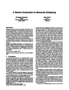
Perceptron vs. L-BFGS in reranking parser 0.91
Averaged perceptron (randomised data) Exponential model, adjusting regularizer constant c
f-score on section 24
0.908
0.906
0.904
0.902
0.9
0.898 0.898
0.9
0.902
0.904
0.906
0.908
0.91
f-score on sections 20-21
52 / 67
Comments on SGD and the Perceptron • Widely used because easy to implement and fast to train É in my experience, not quite as good as numerical optimisation with L-BFGS • Overlearning can be a problem É regularisation becomes weight decay É L 2 regularisation is multiplicative weight decay É L 1 regularisation is subtractive weight decay É often more or less ad hoc methods are used instead of or in addition to regularisation – averaging (bagging, averaged perceptron, etc.) – early stopping
• If you’re using either SGD or Perceptron, try ADAGRAD and ADADELTA
learning rules these methods automatically change the learning rate ε during learning they can identify different learning rates for different features ⇒ much faster learning that with SGD or Perceptron alone É
É
53 / 67
Outline Introducing exponential models Features in exponential models Learning exponential models Regularisation Conditional models Stochastic gradient descent and error-driven learning Avoiding the partition function and its derivatives Weakly labelled training data Summary
54 / 67
Challenges when Y is large • The SGD update rule:
w Ò(t +1) Ew [f | x]
� = w Ò(t ) − ε Ew Ò(t) [f | xrt ] − f (xrt , yrt ) , where: X = f (x, y 0 ) Pw (y 0 | x) y 0 ∈Y
Pw (y | x)
=
Z (x)
=
1 exp (w · f (x, y )) Z (x) X � exp w · f (x, y 0 ) y 0 ∈Y
• Each update step requires calculating the partition function Z (x)
and its derivatives Ew Ò(t) [f | xrt ]
• These require summing over Y, which can dominate the computation time if
Y is large É
in modern speech recognition and machine translation systems, Y is the vocabulary of a natural language, so |Y| ≈ 105
55 / 67
Factoring P(Y | X ) • Produce a hierarchical clustering of Y, which defines a tree over the Y.
• •
•
y1 y2 y3 y4 • Train a separate model for each internal node in the tree É the probability of a leaf (output) node is the product of probabilities of each decision on the root to leaf path • This usually does not produce a very good model • Conjecture: bagging (e.g., averaging) the output of many such tree models
would improve accuracy
56 / 67
Estimating expected feature counts by sampling • SGD update rule:
w Ò(t +1)
� = w Ò(t ) − ε Ew Ò(t) [f | xrt ] − f (xrt , yrt ) , where: X Ew [f | x] = f (x, y 0 ) Pw (y 0 | x) y 0 ∈Y
• Idea: use a sampling method to estimate the expected feature counts
Ew Ò(t) [f | xrt ] • Importance sampling: É É
draw samples from a proposal distribution over Y (e.g., unigram distribution) calculate expectation from samples reweighted according to importance weights (which don’t require partition function)
• May require a large number of samples to accurately estimate expectations
57 / 67
Noise-contrastive estimation • Noise-contrastive estimation can be viewed as importance sampling with only
two samples (and where importance weights are ignored) • Suppose the training item at iteration t is (xrt , yr+ ). t • Set yt− ∈ Y to a random sample from a proposal distribution (e.g., unigram
distribution over Y) • We approximate:
Ew Ò(t) [f | xrt ] ≈
f (xrt , yr+t ) exp(w(t ) · f (xrt , yr+t )) + f (xrt , yt− ) exp(w(t ) · f (xrt , yt− )) exp(w(t ) · f (xrt , yr+t )) + exp(w(t ) · f (xrt , yt− ))
+ • If yt− is less probable than yr+ the expectation Ew Ò(t) [f | xrt ] ≈ f (xrt , yrt ), so t
the expectations will cancel, and there won’t be a large weight update
− • If yt− is more probable than yr+ the expectation Ew Ò(t) [f | xrt ] ≈ f (xrt , yt ), so t
there can be a large weight update
• Widely used in the neural net community today 58 / 67
Outline Introducing exponential models Features in exponential models Learning exponential models Regularisation Conditional models Stochastic gradient descent and error-driven learning Avoiding the partition function and its derivatives Weakly labelled training data Summary
59 / 67
Ambiguous or weakly labelled training data as partial observations • Suppose our training data doesn’t tell us the true label yi for each example xi ,
but only provides us with a set of labels Yi that contains the unknown true label yi D
=
((x1 , Y1 ), . . . , (xn , Yn )) where:
Yi ⊆ Y Qn • Idea: learn a model that maximizes i =1 P(Yi | xi ) yi
∈
• Example: in reranking the gold parse might not be in the beam, so train model
to select one of the best parses available in beam; we don’t care which is chosen • Example: in arc-eager dependency parsing, several different moves can lead to
same gold parse; we don’t care which the parser chooses
60 / 67
Partially-observed conditional exponential models • Data D = (((x1 , Y1 ), . . . , (xn , Yn )), where Yi ⊆ Y and Yi 6= ∅ • Compute maximum conditional likelihood estimator by minimizing negative log
conditional likelihood w Ò = `D (w)
=
argmin `D (w), where: w
−
n X
log Pw (Yi | xi )
i =1
=
n X
(log Z (xi , Y) − log Z (xi , Yi )) , where:
i =1
Z (x, Y 0 )
=
X
� exp w · f (x, y 0 )
y 0 ∈Y 0
• Intuition: log Z (xi , Y) − log Z (xi , Yi ) will be small when most mass is assigned
to Yi • If Yi = Y, then example i has no information • Warning: `D is usually not convex ⇒ local minima É hidden data problems usually have non-convex log likelihoods 61 / 67
Derivatives for partially-observed conditional models • Negative log likelihood:
`D (w)
=
n X
(log Z (xi , Y) − log Z (xi , Yi )) , where:
i =1
Z (x, Y 0 )
X
=
� exp w · f (x, y 0 )
y 0 ∈Y 0
• Derivatives are differences of two conditional expectations
∂`D ∂wj
=
0
=
Ew [fj | x, Y ]
n X
� Ew [fj | xi , Y] − Ew [fj | xi , Yi ] , where:
i =1
X
fj (x, y 0 )Pw (y 0 | x)
(expected value given x and Y 0 )
y 0 ∈Y 0
• These derivatives are no harder to compute than for the fully-observed case • SGD and perceptron algorithms generalise straight-forwardly to
partially-observed data 62 / 67
Partially-observed data in the reranker
• Training data consists of a sequence of training data items (sentences) • Each data item consists of a sequence of candidates (parses) É the number of candidates per data item can vary • Each candidate consists of a sequence of feature-value pairs • Each feature is an integer, and each value is a floating-point number É feature value 1 is special-cased because it’s so common in “one-hot” representations • To allow partially-observed training data, each candidate has a gold weight É for a standard MaxEnt model, the gold candidate in each data item has gold weight 1, all others have gold weight 0 É with partially-observed data, more than one candidate has weight 1
63 / 67
Other interesting things the reranker can do • Data items (sentences) and candidates (parses) can be given “costs” so the
reranker can calculate f-scores É É
can optimise expected f-score instead of log likelihood useful with skewed data (e.g., in disfluency detection, where most words are fluent)
• The reranker uses L1 and/or L2 regularisation É can optimise regulariser constants to maximise log likelihood or f-score of heldout data • Features are organised into feature classes É each feature class can have its own regulariser constant É these feature constants can be optimised can be on heldout data • Standard optimiser is L-BFGS-OWLQN, but can also use Averaged
Perceptron É É
Averaged Perceptron is not quite as good as L-BFGS, but much faster Averaged Perceptron can be used to search for subset of feature classes that optimise f-score on heldout data
64 / 67
Outline Introducing exponential models Features in exponential models Learning exponential models Regularisation Conditional models Stochastic gradient descent and error-driven learning Avoiding the partition function and its derivatives Weakly labelled training data Summary
65 / 67
Summary • Maximum entropy models capture the intuition that features interact
multiplicatively, i.e., can increase or decrease the probability of an outcome • Calculating the partition function Z and its derivatives is usually the central
challenge in MaxEnt modelling • Conditional MaxEnt models, which model P(y | x), often have simpler
partition functions than joint models, which model P(y , x). • Regularisation is often essential to avoid over-learning É L1 regularisation produces sparse feature weight vectors w at the individual feature level É the group Lasso produces sparse feature weight vectors w at the feature group level • Stochastic Gradient Descent (SGD) is an easy and fast way to learn MaxEnt
models (but less accurate?) • The Perceptron is SGD for conditional MaxEnt with a Viterbi approximation
66 / 67
Where we go from here
• Conditional Random Fields are conditional MaxEnt models that use dynamic
programming to calculate the partition function and their derivatives É
generally requires Y to have some kind of regular structure, e.g., a sequence (sequence labelling) or a tree (parsing)
• Neural networks use MaxEnt models as components (they are networks of
MaxEnt models, but “neural net” sounds better!) É É
Boltzmann machines are MaxEnt models where the data items are graphs feed-forward networks use conditional MaxEnt models as components
67 / 67