1
A Geometric Framework to Visualize Fuzzy-clustered Data Yuanquan Zhang† and Luis Rueda∗
Abstract— Fuzzy clustering methods have been widely used in many applications. These methods, including fuzzy k-means and Expectation Maximization, allow an object to be assigned to multi-clusters with different degrees of membership. However, the memberships that result from fuzzy clustering algorithms are difficult to analyze and visualize, and usually are converted to 0-1 memberships. In this paper, we propose a geometric framework to visualize fuzzy-clustered data. The scheme provides a geometric visualization by grouping the objects with similar cluster membership, and shows clear advantages over existing methods, demonstrating its capabilities for viewing and navigating intercluster relationships in a spatial manner. Index Terms— machine learning, fuzzy clustering, clustering visualization, curse of dimensionality.
I. I NTRODUCTION Clustering algorithms have been widely used to discover knowledge in many applications, such as speech, handwriting, medicine, and molecular biology. Quite a few clustering algorithms exist, being the most important ones k-means [1], fuzzy k-means [2], expectation maximization (EM) [3], hierarchical clustering [4], and self-organizing maps [5]. Fuzzy clustering consists of grouping objects which share a certain degree of similarity, by assigning a probability of membership to each cluster. In molecular biology, for example, applying fuzzy clustering to microarray data brings the advantage that the clustering result allows a gene to be assigned to more than one cluster [2], [6]. The problem, however, is how to assign the objects to one of the clusters. A common technique to deal with this is to use a “cutoff” value and assign an object to a cluster, if its membership probability is above the cutoff. On the other hand, visualizing the “fuzzy” membership of an object belonging to different clusters constitutes in itself an open problem. A few simple methods have been proposed in this direction, which we briefly discuss below. Parallel coordinates is a method to visualize highdimensional data in a two dimensional graph [7], [8], [9]. Roughly speaking, parallel coordinates represent a high-dimensional object, say n-dimensional data, as a line that crosses n parallel axes in a two dimensional graph. Usually, the distance between two axes is fixed to unity. † School of Computer Science, University of Windsor, 401 Sunset Ave., ON, N9B 3P4, Canada. E-mail:
[email protected]. ∗ Member of the IEEE. School of Computer Science, University of Windsor, 401 Sunset Ave., Windsor, ON N9B 3P4, Canada. E-mail:
[email protected]. Phone +1-519-253-3000 Ext. 3780, Fax +1-519-9737093.
Figure 1 shows an example in which three 4-dimensional objects are visualized using parallel coordinates. Although parallel coordinates are capable of visualizing data in a lower-dimensional space, the plots become rather confusing when the dimension of the original space is large. In [10], the authors propose a method to visualize fuzzy points in each dimension in detail. They point out the disadvantage that the existing fuzzy-point techniques only show centroids or use shaded areas to represent the variance of cluster centers. An extended version of parallel-coordinates visualization is to apply color shading for representing the degree of membership. The advantage of the approach is that it allows users to observe overlapping areas through different degrees of shading. This scheme is not able to show the area where many clusters overlap. Since each cluster is represented by a shading area in different colors in the visualization, the overlapping area is a color-mixed area. Thus, when the number of clusters is large, the visualization will fail to compare the fuzzy clustered results of the clusters. In addition, the shading function they use in the visualization is linearly decreased from the centroid of the cluster. There is no guaranty that an object with lower membership will always be located farther than an object with higher membership from the mean of the cluster over all axes. Moreover, given such a visualization, it is difficult to predict the correlation of objects. For example, it is hard to estimate whether an object has a higher membership than another from the visualization. Gasch et al. proposed a modified hierarchical visualization to observe the fuzzy-clustered genes utilizing different membership cutoff values [11]. In the membership table, each objects can be related to all the identified clusters through its membership value. As a consequence of this, all the objects can be ranked in different continuous lists for each cluster based on their membership values. The method then uses a “cutoff” membership value to restrict the objects which are displayed for a given cluster. All objects whose membership is greater than the “cutoff” value are selected as part of the given cluster. Instead of using a unique cutoff value, they define different cutoff values for each cluster to yield a more accurate visualization. However, in their visualization, all objects are plotted along one dimensional axis, and hence it is not possible to compare the level of similarity between one cluster and other clusters which are not plotted next to that cluster in the visualization. Also, this method is not able to visualize the distances (similarity) between two clusters, and
2
against other clusters.
A few observations are in place. Based on Definition 3, k-means is a fuzzy clustering algorithm, thought it produces a 0-1 membership matrix. Thus k-means is a special case of fuzzy clustering, which also satisfies the definition of fuzzy clustering. However, the clustering result of k-means is not “fuzzy” or “soft” in the strict sense.
7
6
5
4
3
2
1
1
1.5
2
2.5
3
3.5
4
Fig. 1. Examples of visualizing three 4-dimensional objects using parallel coordinates.
In [12], we have shown that fuzzy-clustered yeast microarray data can be visualized in a spatial manner using a 4vertex tetrahedron. In this paper, we propose a geometric visualization framework that visualizes higher-dimensional data on a lower-dimensional space given by the number of clusters. Our approach projects the fuzzy membership data onto a hyper-tetrahedron, which allows to observe the intercluster relationships in a spatial manner. We show the results of visualizing fuzzy clustered data for synthetic and real-life datasets.
p1 0.12 0.82 0.01 .. . 0.01
ω1 ω2 ω3 .. . ωk
p2 0.78 0.07 0.03 .. . 0.08
p3 0.11 0.09 0.14 .. . 0.69
... ... ... ... .. . ...
pn 0.01 0.07 0.56 .. . 0.04
TABLE I A N EXAMPLE OF A MEMBERSHIP MATRIX
Given a dataset, D = {x1 , x2 , . . . , xn }, and k, fuzzy kmeans seeks a minimum of a heuristic global cost function: Jf uz =
k X n X [Pˆ (ωj |xi )]b d(xi , µj )
,
(1)
j=1 i=1
where b is a “fuzziness” parameter, which is greater than unity, n X [Pˆ (ωj |xi )]b xi
µj =
i=1 n X
,
(2)
[Pˆ (ωj |xi )]b
II. F UZZY C LUSTERING i=1
Fuzzy clustering, also called “soft” clustering, assigns each sample to multiple clusters using a membership value, which is the probability of the sample belonging to the corresponding cluster. Various methods use this idea, being the most widely used ones, fuzzy k-means and expectation maximization [3]. Before discussing these clustering algorithms, the following definitions are introduced. Consider a dataset D = {x1 , x2 , . . . , xn } where xi = [xi1 , xi2 , . . . , xip ]t is a p-dimensional feature vector that represents a sample (object), and xir is the rth feature of xi . Also, consider a set of k unknown classes (clusters) {ω1 , . . . , ωk }. Definition 1: mi = [m1i , . . . , mki ]t ∈ Rk is a membership vector, if 0 ≤ mji ≤ 1 represents the probability that xi k X belongs to cluster ωj , 1 ≤ j ≤ k, and mji = 1, where k j=1
is the number of clusters. Definition 2: A membership matrix, M , is a matrix composed of n membership vectors, i.e. M = [m1 , . . . , mn ]. Definition 3: Given a dataset D = {x1 , x2 , . . . , xn }, and a number of clusters, k, a fuzzy clustering algorithm is a method that receives D and k as input, and produces a membership matrix.
is the cluster center of ωj Pˆ (ωj |xi ) =
(1/dji )1/(b−1) k X (1/dri )1/(b−1)
,
(3)
r=1
is the probability that xi is assigned to cluster ωj , and d is a distance function. Fuzzy k-means proceeds in an iteratively manner. It receives k and b as parameters, and initializes µ1 , . . . , µk , and Pˆ (ωj |xi ), where i = 1, . . . , n, j = 1, . . . , k. It then iteratively recomputes µj and Pˆ (ωj |xi ) using (2) and (3) until small changes in µj and Pˆ (ωj |xi ) are observed. The resulting membership matrix is given by mjr = Pˆ (ωj |xi ) for i = 1, . . . , n, j = 1, . . . , k. An example of such a membership matrix is given in Table I. Another criterion that can be optimized, instead of (1), is to maximize the likelihood that a sample belongs to ωj with a probability given by a mixture of densities. In such a case, the aim is to estimate the parameters, say a vector ˆ = [θˆ1 , . . . , θˆk ], while maximizing the likelihood. A comθ mon strategy is to assume that the samples were generated from a mixture of k-dimensional normal distributions. In this case, the parameter to be estimated are k mean vectors, ˆ 1, . . . , Σ ˆ k }. A ˆ 1, . . . , µ ˆ k }, and k covariance matrices, {Σ {µ common approach used in optimizing this criterion is the EM algorithm [13], [14], which works as follows. First, initialize
3
ˆ j , where j = 1, . . . , k. Then, iterate the ˆ j and Σ Pˆ (ωj |xi ), µ following two steps until convergence to a local maximum of the likelihood function is achieved. 1) E-Step: ˆ Pˆ (ωj |xi , θ) =
ˆ Pˆ (ωj ) p(xi |ωj , θ) k X ˆ Pˆ (ωr ) p(xi |ωr , θ)
Definition 6: A regular k-vertex is a µ hyper-tetrahedron ¶ k hyper-tetrahedron in which all the 1-faces have same 2 length.
(4) A regular hyper-tetrahedron can be intuitively constructed by choosing a point in a higher dimension, which is equidistant to all the vertices in the current dimension, and is connected to all the current vertices. The generation steps are shown in Figure 2.
r=1 −1
=
Definition 5: An i-face is a hyper-tetrahedron of i + 1 vertices.
ˆ ˆj) ˆ ˆ j |− 12 e− 12 (xi −µˆ j )t Σ j (xi −µ |Σ P (ωj ) , k X ˆ −1 (xi −µ ˆ r )t Σ ˆr) ˆ − 12 − 21 (xi −µ ˆ r P (ωr ) |Σr | e r=1
2) M-Step: n X
ˆj = µ
ˆ i Pˆ (ωj |xi , θ)x
i=1 n X
,
(5)
ˆ Pˆ (ωj |xi , θ)
i=1 n X
ˆj = Σ
Fig. 2. Generation of a hyper-tetrahedron from the one-dimensional space to the three-dimensional space.
ˆ i−µ ˆ j )(xi − µ ˆ j )t Pˆ (ωj |xi , θ)(x
i=1 n X
,
(6)
ˆ Pˆ (ωj |xi , θ)
i=1 n
1Xˆ ˆ Pˆ (ωj ) = P (ωj |xi , θ) n i=1
,
(7)
ˆ Finally, a membership table, given by mji = Pˆ (ωj |xi , θ), is obtained, where mji represents the probability that sample, xi , belongs to cluster ωj .
It is opportune to note that a regular k-vertex hypertetrahedron is a convex polytope in (k − 1)-dimensional space [15]. Therefore, all the edges of the regular hyper-tetrahedron have the same length. Otherwise, a k-vertex convex polytope is called irregular hyper-tetrahedron. We assume that a k-vertex irregular hyper-tetrahedron is always a k-vertex convex polytope. Figure 3 shows an example of regular and irregular hyper-tetrahedrons of 4 vertices, where points m00 and m000 are inside the regular and irregular hyper-tetrahedrons respectively.
III. T HE G EOMETRIC V ISUALIZATION S CHEME To understand the relationships among objects and their memberships to the clusters, we propose a visualization framework on the fuzzy clustered results. To achieve this, a geometric model, that uses a hyper-tetrahedron, is utilized. The location of the objects in the hyper-tetrahedron is obtained using concepts from geometry. Finally, a visualization which presents the fuzzy relationships of the objects is obtained. A. Properties of fuzzy memberships In order to geometrically visualize objects by using their memberships, we, first of all, define the hyper-tetrahedron, in which all objects will be projected. We then show that the membership vectors can be placed inside a hyper-tetrahedron based on their barycentric coordinates [15], [16]. Definition 4: A k-vertex hyper-tetrahedron, Tk = [y 1 , . . . , y k ]t , is an n-simplex, where n = k − 1, which µ ¶ k has a boundary given by all i-faces, where i+1 i = 0, . . . , k − 1.
Fig. 3.
Examples of regular and irregular hyper-tetrahedrons of 4 vertices.
To establish the relation between the membership matrix and the hyper-tetrahedron, we now introduce the following definition [15], [16]: Definition 7: Let Tk = [y 1 , . . . , y k ]t be a k-vertex hypertetrahedron. A point p is inside Tk , and there exists a series of numbers, or the vector [t1 , . . . , tk ]t , called barycentric coordinates with respect to the vertices of Tk , if the following properties are satisfied:
4
(i) tj ≥ 0, (ii)
k X
j = 1, . . . , k
tj = 1, and
,
(8)
(9)
j=1
(iii) p=
k X
tj y j
.
(10)
j=1
Note that a point p, which has barycentric coordinates referring to all vertices, is inside the hyper-tetrahedron defined by those vertices. The barycentric coordinates of the point are invariant to both rotations and translations because of the definition given in [17], [18]. In addition, the barycentric coordinates can also be treated as weights placed at the vertices so that p becomes the center of gravity of all vertices. The coordinates of p, which is inside a hyper-tetrahedron, can thus be obtained using (10). Lemma 1: Every membership vector mi = [m1i , m2i , . . . , mki ]t contains its barycentric coordinates in a hyper-tetrahedron Tk = [[1, 0, ..., 0]t , [0, 1, ..., 0]t , . . . ,[0, 0, ..., 1]t ]t . Proof: The proof follows from Definitions 1 and 7, and from the fact that vertices, [1, 0, ..., 0]t , [0, 1, ..., 0]t , . . . ,[0, 0, ..., 1]t , conform an orthogonal basis in Rk . The complete proof can be found in [19]. For example, in Figure 4 (a), m is a point inside a 2vertex hyper-tetrahedron defined by [1, 0]t and [0, 1]t , where the barycentric coordinates of m are [m1 , m2 ]t . In Figure 4 (b), m is a point inside a 3-vertex hyper-tetrahedron defined by [1, 0, 0]t , [0, 1, 0]t and [0, 0, 1]t , where the barycentric coordinates of m are [m1 , m2 , m3 ]t .
1) Obtaining Vertices of the Regular Hyper-tetrahedron: As shown in Lemma 1, the membership vectors m1 , . . . , mn lie in the k-dimensional space, where the j th cluster, ωj , is represented by a k-dimensional vector y j = [yj1 , . . . , yjk ]t with yjr = 0 for r = 1, . . . , k, r 6= j and yjj = 1. Therefore, a k-dimensional membership vector mi is inside the (k − 1)-dimensional regular hyper-tetrahedron defined by Y . The first step is to project the vertices of a regular hypertetrahedron, which conform a (k − 1)-dimensional hyperplane in the original k-dimensional space, onto a new k-vertex hyper-tetrahedron in the (k − 1)-dimensional space, where the k clusters are represented by k points, y 01 , . . . , y 0k in the new space. These points compose a new hyper-tetrahedron defined by Y 0k = [y 01 , . . . , y 0k ]t . Since the distances between each pair of vertices are the same for all pairs, we can reconstruct the vertices in k − 2 iterations. In each step, √ we add a new vertex, which has a unique distance, say 2, to other vertices which are already obtained. In this case, the Euclidean distance between each pair of vertices is not changed after the transformation. Here, the initialization √ is done in such a way that the first two vertices, [0, 0] and [ 2, 0] are already given. The algorithm is given below. · ¸ 0 0 Step 1. Initialize Y 02 ← √ . 2 0 Step 2. Let Y = 0 j
D 0j
Fig. 4. Examples of hyper-tetrahedrons, a point, and its corresponding barycentric coordinates.
B. Creating a Regular Hyper-tetrahedron The geometric visualization approach takes the membership matrix (generated by a fuzzy clustering algorithm) as input and perform three different stages. The first stage finds the k vertices of a regular hyper-tetrahedron, onto which all the n membership vectors are projected. The process finally transforms the regular tetrahedron into an irregular one that reflects the inter-cluster centroid distances.
0 0 y21 0 y31 .. .
0 0 0 y32 .. .
0 0 0 .. .
... ... ... .. .
0 0 0 .. .
0 yj1
0 yj2
...
0 yj(j−1)
0
d013 d023 .. .
d012 0 .. .
0 0 .. .
= 0 0
0 0
0 0
,
(11)
... ... .. .
d01j d02j .. .
... ...
d0(j−1)j
,
(12)
0
where y j = [yj1 , yj2 , . . . , yjk ]t . Step 3. Assume that the distance from y 0j+1 to y 01 , y 02 , . . . , y 0j is given by a j-dimensional vector d0j+1 = [d0(j+1)1 , d0(j+1)2 , . . . , d0(j+1)j ]t . √ √ √ We set d0j+1 ← [ 2, 2, . . . , 2]t , since those√ vertices compose a hyper-tetrahedron whose edge length is 2 in the j-dimensional space. Then, y 0j+1 is computed as follows: 0 0 [y(j+1)1 , . . . , y(j+1)(j−1) ]t ←
where
y 0s =
1 0 ˆ Y (d + y 0s ) , 2 c
0
0
y212 0 0 2 y31 + y322 .. .
0
(13)
0
2 yj12 + yj22 + . . . + yj(j−1)
,
(14)
5
Y = 0 c
0 y21 0 y31 .. .
0 y32 .. .
... ... .. .
0 0 .. .
yn1
yn2
...
yn(n−1)
,
and
(15)
dˆ = [d2v1 − d2v2 , d2v1 − d2v3 , . . . , d2v1 − d2vn ]t .
(16)
0 Step 4. The last component of y 0j+1 , y(j+1)j , is computed as below: q 02 02 02 0 . (17) y(j+1)j = d(j+1)1 − y(j+1)1 . . . − y(j+1)(j−1)
As a result, we obtain a j-dimensional vector, y 0j+1 . Step 5. Transform y 01 , . . . , y 0j+1 into (j + 1)-dimensional vectors as follows: y 0r ← [(y 0r )t , 0]t , where r = 1, . . . , j + 1, and update Y 0 as: Y 0 ← [y 01 , . . . , y 0r ]t , where r = 1, . . . , j+1. Step 6. If j + 1 = k, stop. Otherwise, go to Step 2. 2) Projecting Vectors onto a Regular Hyper-tetrahedron: The vectors in M can be seen as points lying in the kdimensional space and the aim now is to transform each point mi = [m1i , . . . , mki ]t into a new point, m0i , which is enclosed in a regular hyper-tetrahedron in the (k − 1)-dimensional space, whose vertices are given by Y 0 . For example, for k = 3,the points will lie on T3 , an equilateral triangle, and 0 0 √0 Y 0 = √ 2 √0 0 . 2 6 0 2 2 Based on the definition of barycentric coordinates and Lemma 1, for all i = 1, . . . , n, m1i , m2i , . . . , mki are the barycentric coordinates of mi , which is inside a hypertetrahedron defined by y 1 = [1, 0, ..., 0]t , y 2 = [0, 1, ..., 0]t , . . . ,y k = [0, 0, ..., 1]t in the k-dimensional space. After reconstructing the new hyper-tetrahedron in the regular space, the new coordinates of the mi , denoted by m0i in the new space, are given by the same barycentric coordinates as mi . Therefore, m0i can be obtained using its barycentric coordinates as follows: k X m0i = mji y 0j , (18) j=1
As a result, we obtain all points m01 , . . . , m0n , which are (k − 1)-dimensional points enclosed in a hyper-tetrahedron given by vertices y 01 , . . . , y 0k . This is stated and proved in the following lemma, whose proof can be found in [19]. Lemma 2: For all i = 1, . . . , n, m0i is inside Tk0 , defined by Y 0 = [y 01 , . . . , y 0k ]t .
coincides with the distance in the regular hyper-tetrahedron. √ d Therefore, d00ij = 2 d00ij , for 1 ≤ i ≤ k, 1 ≤ j ≤ k, 12 results in a distance relative to d0012 . Thus, Y 00j and D 00j have the same form as Y 0j and D 0j . Here, we assume that the k-vertex irregular hyper-tetrahedron obtained is a k-convex polytope with k vertices, otherwise we may obtain overlapping points, which will not obey the definition of the barycentric coordinates. Therefore, a visualization using a regular tetrahedron is a better solution in this case. To obtain the vertex coordinates of the irregular hypertetrahedron, we apply a procedure similar to the algorithm described in Section III-B.1, except that vectors y 01 , . . . , y 0n are transformed into vectors y 001 , . . . , y 00n lying in an irregular tetrahedron. In addition, the distance vector, d00j+1 is computed as above, i.e. d00j+1 = [d00(j+1)1 , d00(j+1)2 , . . . , d00(j+1)j ]t , where √ d d00ij = 2 d00ij , for 1 ≤ i ≤ k, 1 ≤ j ≤ k. 12 To reflect the distances between each pair of vertices in the visualization, the points in the regular hyper-tetrahedron are “stretched” along a series of steps, which depend on the distance values. The distance between two vertices also depends on the distance between the centroids of the two clusters represented by the corresponding two vertices in the hyper-tetrahedron. All the points inside the hyper-tetrahedron that includes all vertices are “shifted” together. 2) Projecting Vectors onto an Irregular Hyper-tetrahedron: The transformed coordinates of the n vertices of the hypertetrahedron are contained in Y 00k , which has the same form as Y 0k . Note that y 001 = [0, . . . , 0]t , which implies that the vertex is located in the origin of the coordinate system. Because the barycentric coordinates determine the relationship between the point and all vertices, a mapped point, m00i , corresponds to the point mi in the original space. The coordinates for point m00i are computed in the same way as computing m0i using the barycentric coordinates, as follows: m00i =
k X
mji y 00j
,
(19)
j=1
The following lemma, whose proof can be found in [19], demonstrates that the new points are inside the irregular hypertetrahedron. Lemma 3: For all i = 1, . . . , n, m00i is inside Tk00 , defined by Y 00 = [y 001 , . . . , y 00k ]t . D. Visualizing a Subset of Clusters
C. Creating an Irregular Hyper-tetrahedron 1) Obtaining the Vertices of an Irregular Hypertetrahedron: To enhance the visualization, we want to show the points in an irregular hyper-tetrahedron that uses the corresponding edges to reflect the inter-cluster distances. Let D 00 be a k × k matrix that contains the distances between each pair of vertices, where dij , i, j = 1, . . . , k and i < j, represents the distance from the centroid of the ith cluster to the centroid of the jth cluster. The values of dij depend on the specific distance function used in the fuzzy clustering algorithm. To avoid extremely large distance values√that may result from certain real-life problems, we let d0012 = 2 which
In real-life, it is practical to visualize a tetrahedron in the three-dimensional space. When dealing with a large set of clusters, it is then convenient to visualize a subset of these clusters. For this purpose, we follow an approach that projects the vectors from a higher-dimensional space to a lower-dimensional space. The projection is used to reduce the n dimensions to the specified lower-dimensional space (usually two or three-dimensional space). The solution is summarized in the following three steps: (1) Extract all membership values which belong to the selected clusters, composing new unnormalized membership vectors. (2) Normalize the resulting vectors so that they satisfy the
6
properties of a membership vector. (3) Visualize the resulting sub membership matrix using the scheme presented in Sections III-B and III-C. This visualization will focus only on a portion of the clustering results, which helps to visualize and understand the relationships of a specific subset of clusters. In addition, we assume that the selected clusters construct a convex polytope in a lower-dimensional space, using similar assumptions to the ones used during the irregular hyper-tetrahedron transformation (Section III-C). Consider the membership matrix in Table II, for example, if we want to visualize only a subset of clusters, ω2 and ω4 , the membership values (in bold) in Table II are first extracted, obtaining Table III. Table IV is obtained after the normalization is applied to Table III. Finally, the visualization scheme proceeds using Table IV. ω1 ω2 ω3 ω4
p1 0.12 0.82 0.05 0.01
p2 0.78 0.07 0.07 0.08
p3 0.11 0.09 0.11 0.69
... ... ... ... ...
TABLE II T HE ORIGINAL MEMBERSHIP TABLE FOR 4
ω2 ω4
p1 0.82 0.01
p2 0.07 0.08
p3 0.09 0.69
... ... ...
(a) Visualization of 3 out of 5 clusters
pm 0.01 0.56 0.39 0.04 CLUSTERS .
pm 0.56 0.04
TABLE III T HE NEW MEMBERSHIPS AFTER CLUSTERS ω2
ω2 ω4
p1 0.99 0.01
p2 0.46 0.54
p3 0.12 0.88
AND
... ... ...
ω4
ARE SELECTED .
pm 0.93 0.07
TABLE IV T HE NORMALIZED MEMBERSHIP TABLE .
IV. S IMULATIONS ON R EAL - LIFE DATA The visualization scheme presented in this paper was applied to two data sets: the Ecoli dataset [20] and the serum dataset [21]. Simulations on the Iris dataset and the yeast dataset can be found in [12]. The visualization is presented in the three-dimensional space and shows the distribution of the fuzzy-clustered data which were clustered into four classes. For each data set, the three-class and four-class visualization are described in following sections. In our simulations, we use fuzzy k-means and the Euclidean distance, which is computed as d(xi , µj ) = ||xi − µj ||2 , and the Pearson Ppcorrelation, which is computed as d(xi , µj ) = 1 − µj ) jr −¯ √Pk−1 r=1 (xik −¯x√i )(µ , where x ¯i is the mean of Pp 2 2 xi ) k=1 (xir −¯
µj ) r=1 (µjr −¯
xi1 , . . . , xip and µ ¯i is the mean of µi1 , . . . , µip . A. The Ecoli Dataset The Ecoli dataset contains 336 protein sequences that belong to one of eight classes. We selected the first 5 classes
(b) Visualization of 4 out of 5 clusters Fig. 5. Visualization of a subset of fuzzy 5-means clustering results using the Ecoli data set.
which contain most of the samples, namely cytoplasm (143), inner membrane without signal sequence (77), perisplasm (52), inner membrane with uncleavable signal sequence (35), and outer membrane (20). First of all, fuzzy 5-means clustering was applied to the selected dataset using the Euclidean distance to compute the distance between each pair of samples. As discussed in Section III-D, to visualize a subset of fuzzy clustering result of higher-dimensional space, we selected 3 and 4 clusters and normalized the membership vectors. A visualization of a subset of 3 out of 5 classes is shown in Figure 5 (a). Another visualization of a subset of 4 classes is shown in Figure 5 (b). From these two visualizations, we can easily observe the relationships between objects and clusters, and interpret the fuzzy memberships of the objects, even though the original data is five-dimensional. In these figures, only the points lying in the irregular tetrahedron are plotted. This means that the figures are “stretched” depending on the corresponding distance between each pair of cluster centroids. Different point patterns were used to distinguish the clusters to which the point most likely belongs. There are four different patterns representing four areas of the tetrahedra. A point inside one area has a higher membership to the corresponding cluster than its membership to other clusters.
7
(a) Visualization of 3 out of 5 clusters
(a) Visualization using Euclidean distance
(b) Visualization of 4 out of 5 clusters
(b) Visualization using Pearson correlation
Fig. 6. Visualization of a subset of EM clustering results using the Ecoli data set.
Fig. 7. Visualization of a subset (3 out of 10 clusters) of fuzzy 10-means clustering results using the Serum data set.
In order to further demonstrate the capabilities of our visualization method, we applied EM to fuzzy cluster the Ecoli dataset. As in the case of visualizing fuzzy k-means, Figure 6 (a) shows the hyper-tetrahedron that contains samples of 3 out of 5 classes, and Figure 6 (B) shows visualization of 4 out of a total of 5 classes. In the two figures, we observe that although most of the objects are very close to the vertices, as a result of applying the EM algorithm, those objects which are relatively far from the vertices can be easily identified.
more reliable clustering result. The distribution of the points in the visualization of the clustering result applying the Euclidean distance has the form of a nearly flat triangle. Note that we have reduced the viewing range in order to avoid this situation. An additional observation is that the distribution of the points in the visualization of the clustering result using the correlation distance sparsely appear inside the tetrahedra, thus, enhancing their visualization.
B. The Serum Dataset This serum dataset is described and used in [21], which contains 517 genes whose expression vary in response to serum concentration in human fibroblasts; each sample is 18dimensional. We apply fuzzy 10-means on the dataset and fuzzy parameter is set to 1.25, which are the same parameters used in [2]. Figure 7 (a) shows the visualization of a subset of 3 out of 10 classes which results from fuzzy 10-means using Euclidean distance. Another visualization of a subset of 3 classes is shown in Figure 7 (b), which visualize the partial results obtained from fuzzy 10-means using the Pearson correlation distance. In addition, we also obtain visualizations of 4 out of 10 classes which are shown in Figure 8 (a) and Figure 8 (b). Regarding the comparison between the Euclidean distance and the correlation distance visualizations, the latter provides a
V. C ONCLUSION We have presented a geometric framework to visualize fuzzy-clustered data that comes from the cluster membership table. The scheme provides a wise visualization of the probability of a point belonging to each cluster, that represents the geometric distribution in the two and three-dimensional spaces. A point with a higher cluster membership appears close to the cluster centroid which is represented as a vertex in the tetrahedron. In addition, the closer the distance between two points is, the more similar the two points are. It is important to emphasize that a short distance between two points in the visualization means that these two points have much more similar cluster membership as a result of fuzzy k-means clustering based on a particular distance function. We have also shown how extract a subspace of the clustered data, which allows the user to visualize sub-sets of classes
8
(a) Visualization using Euclidean distance
(b) Visualization using Pearson correlation Fig. 8. Visualization of a subset (4 out of 10 clusters) of fuzzy 10-means clustering results using the Serum data set.
and project them onto the two or three-dimensional space. We have demonstrated the capabilities of our geometric visualization framework on real-life biological data, whose original dimension is large, up to 18. R EFERENCES [1] S. Theodoridis and K. Koutroumbas, Pattern Recognition, 2nd Edition, Academic Pr, 2003. [2] D. Dembele and P. Kastner, “Fuzzy C-means Method for Clustering Microarray Data,” Bioinformatics, vol. 19, no. 8, pp. 973–80, May 2003. [3] R. Duda, P. Hart, and D. Stork, Pattern Classification, 2nd Edition, John Wiley and Sons, Inc., New York, NY, 2000. [4] M. Eisen, P. Spellman, P. Brown, and D. Botstein, “Cluster Analysis and Display of Genome-Wide Expression Patterns,” Proceedings of the National Academy of Sciences, USA, vol. 95, pp. 14863–14868, 1998. [5] T. Kohonen, The Self-Organizing Maps, 3rd Edition, Springer-Verlag, 2001. [6] M. E. Futschik and N. K. Kasabov, “Fuzzy Clustering of Gene Expression Data,” World Congress of Computational Intelligence WCCI, vol. 1, pp. 414–419, 2002. [7] A. Inselberg, “n-dimensional graphics, part i–lines and hyperplanes,” Technical report g320-2711, IBM Los Angeles Scientific Center, IBM Scientific Center, 9045 Lincoln Boulevard, Los Angeles (CA), 900435, 1981. [8] A. Inselberg, “Multidimensional detective,” IEEE Symposium on Information Visualization, InfoVis, p. 100C107, 1997. [9] A. Inselberg and T. Avidan, “The Automated MultidimensionalDetective,” IEEE Symposium on Information Visualization, 1999. [10] M. R. Berthold and L. O. Hall, “Visualizing Fuzzy Points in Parallel Coordinates,” Fuzzy Systems, vol. 11, pp. 369–374, June 2003.
[11] A. P. Gasch and M. B. Eisen, “Exploring the Conditional Coregulation of Yeast Gene Expression through Fuzzy k-means Clustering,” Genome Biology, vol. 3, no. 11, pp. 1–22, 2002. [12] L. Rueda and Y. Zhang, “Geometrically Visualizing Microarray Time Series Experiments Clustered with Fuzzy k-Means,” WSEAS Transactions on Biology and Biomedicine, vol. 2, pp. 133–140, 2005. [13] A. Dempster, N. Laird, and D. Rubin, “Maximum likelihood from incomplete data via the EM algorithm,” Journal of the Royal Statistical Society, Series B, vol. 39, no. 1, pp. 1–38, 1977. [14] H. Hartley, “Maximum Likelihood Estimation from Incomplete Data,” Biometrics, , no. 14, pp. 174–194, 1958. [15] H. S. M. Coxeter, Introduction to Geometry, 2nd ed., chapter 13.7 Barycentric Coordinates, pp. 216–221, New York: Wiley, 1969. [16] Joe Warren, “Barycentric Coordinates for Convex Polytopes,” Advances in Computational Mathematics, vol. 6, pp. 97–108, 1996. [17] Branko Grunbaum, Victor Klee, M.A. Perles, and G.C. Shephard, Convex Polytopes, New York: Wiley, 1967. [18] Mark Meyer, Alan Barr, Haeyoung Lee, and Mathieu Desbrun, “Generalized barycentric coordinates on irregular polygons,” Journal of Graphics Tools, vol. 7, no. 1, pp. 13–22, November 2002. [19] Y. Zhang, “On the Visualization of Fuzzy Clustered data,” M.S. thesis, School of Computer Science, University of Windsor, 2005, In preparation. Electronically available at http://www.cs.uwindsor.ca/˜lrueda/papers/KenThesis.pdf. [20] C.L. Blake and C.J. Merz, “UCI Repository of Machine Learning Databases,” 1998. [21] V.R. Iyer and M.B. Eisen et. al., “The transcriptional program in the response of human fibroblast to serum,” Science, vol. 283, no. 5398, pp. 83–87, 1999.