A geometrically regularized gradient-damage model ...

Available online at www.sciencedirect.com

ScienceDirect Comput. Methods Appl. Mech. Engrg. 328 (2018) 612–637 www.elsevier.com/locate/cma

A geometrically regularized gradient-damage model with energetic equivalence Jian-Ying Wu State Key Laboratory of Subtropical Building Science, South China University of Technology, 510641 Guangzhou, China Received 26 January 2017; received in revised form 18 June 2017; accepted 19 September 2017 Available online 2 October 2017 Dedicated to Prof. Jie Li on the occasion of his 60th birthday

Highlights • • • • •

A geometrically regularized gradient-damage model with energetic equivalence is proposed. The damage evolution law emerges from the geometric regularization and energetic equivalence. The crack is implicitly represented, and cumbersome crack tracking strategies are not required. The length scale can be regarded either as a small numerical parameter or as a material property. The localization bandwidth approaches to a finite limit value, not exhibiting spurious damage growth.

Abstract Aiming to bridge the gap between damage and fracture mechanics for modeling localized failure in solids, this paper addresses a novel geometrically regularized gradient-damage model with energetic equivalence for cracking evolution. With the free energy potential defined as usual in terms of the local strain and damage fields, the constitutive relations are derived consistently from the standard framework of thermodynamics. Upon the sharp crack topology geometrically regularized by the damage localization band with a length scale, the ensuing energetic equivalence naturally yields the damage evolution law of gradient-type and the associated boundary condition of Neumann-type. Compared to other gradient-damage models, no extra assumptions like the nonlocal energy residual and insulation condition are introduced. Moreover, the damage gradient, physically accounting for microscopic nonlocal interactions, is fully dissipative as expected. In line with the unified phase-field theory recently proposed by the author (Wu, 2017) during failure processes the material behavior is uniquely characterized by two constitutive functions, i.e., the degradation function defining the free energy potential of the bulk and the geometric function regularizing the sharp crack topology. In particular, optimal constitutive functions defining an equivalent cohesive zone model of general softening laws are postulated, with the involved parameters calibrated from standard material properties. The proposed model is numerically implemented into the multi-field finite element method and applied to several benchmark tests of concrete under mode-I and mixed-mode failure. It is found that the incorporated length scale can be regarded either a numerical parameter or a material property. For the former considered in this work, the length scale has negligible, if not no, effects on the global responses, so long as the sharp crack topology and the damage field of high gradients within the localization band are well resolved. Furthermore, the localization bandwidth does not exhibit spurious widening, but rather, it approaches to a finite value proportional to the length scale. Comparison between E-mail address: [email protected]. https://doi.org/10.1016/j.cma.2017.09.027 c 2017 Elsevier B.V. All rights reserved. 0045-7825/⃝

J.-Y. Wu / Comput. Methods Appl. Mech. Engrg. 328 (2018) 612–637

613

the numerical and experimental results, regarding the curve of load versus displacement and crack path, confirms validity of the proposed gradient-damage model for characterizing localized failure in quasi-brittle solids. c 2017 Elsevier B.V. All rights reserved. ⃝

Keywords: Quasi-brittle solids; Localized failure; Gradient-damage model; Phase-field theory; Damage; Fracture

1. Introduction Onset of macroscopic failure in solids and structures is generally preceded by highly localized non-uniform deformations (i.e., strain localization) within bands of small (or surfaces of negligible) width compared to the structural size. Inside and outside these localized domains, the strain field is either discontinuous due to continuous but non-smooth displacements or even singular (unbounded) caused by displacement discontinuities. Being such localized failure regarded as prognostics of catastrophic collapse of structures, it is of vital importance to predict its occurrence and quantify its adverse effects on overall structural responses. Ever since the pioneering work of Ngo and Scordelis [1] and Rashid [2], a large volume of theoretical models based on fracture and damage mechanics have been proposed to characterize material behavior with softening regimes. Meanwhile, various computational approaches like the smeared and discrete crack methods have also been developed. However, just as commented by Prof. Baˇzant in the Speech of Acceptance of the 2009 Timoshenko Medal: “The mechanics of damage and quasi-brittle fracture, with its scaling and interdisciplinary coupling, is a problem of the same dimension (as turbulence), which will not be closed even a century from now”, the modeling of localized failure in solids and structures is still an opening issue. Among many others, the most stringent challenge arises when those theoretical models and computational methods are implemented into the numerical (discrete) context, e.g., the finite element method (FEM) or other alike. On the one hand, owing to the lack of a well-defined length scale and the loss of ellipticity in the governing equations, local material models with softening regimes cannot be used straightforwardly in the numerical context; otherwise, mesh dependent and misleading results would be unavoidable [3,4]. In order to circumvent such issues, non-local and gradient-enhanced damage models [5,6] have been proposed. With a nonlocal damage driving force defined either in integral or gradient form, a material length scale is introduced to restore well-posedness of the resulting (initial) boundary value problem. However, the boundary effect related to the integral form [7] and the boundary condition for the gradient form [8] cannot be easily dealt with. Even worse, as a constant interaction domain allows the energy transferring from the fracture process zone to neighboring regions in elastic unloading, non-local and gradientenhanced damage models tend to diffuse the localization band [9], leading to spurious damage growth. Consequently, localized deformations are precluded due to this ‘damage diffusion’ process, giving erroneous numerical predictions in mode-I failure and shear band problems [10]. Interesting remedies include the ‘over-nonlocal’ formulation [11,12] and nonlocal models with stress-based weighting functions [13], decreasing interactions [14] or evolving length scale [15], etc.; see [16] and the references therein. On the other hand, due to the intrinsic kinematic deficiency and a priori limitation of crack propagation paths, respectively, the classical smeared and discrete crack methods suffer from the issues of mesh-alignment dependence and spurious stress locking [3,17]. In order to restore objectivity of the numerical solution, the more powerful enriched FEM, e.g., the embedded FEM [18] and extended FEM [19], etc., were proposed; see [20,21] for the reviews. With the discontinuity kinematics enhanced and the solution space enriched, such advanced numerical methods allow cracks propagating arbitrarily intra-elements and stress locking-free states can be achieved for a fully softened crack, provided the crack path is well tracked during the entire failure process. However, the numerical issues related to the ill-conditioned system matrix [22], oscillations in tractions [23], quadrature of discontinuous functions [24], etc., limit the application of such methods, though some remedies like the stable XFEM [25,26], the regularized XFEM [27], etc., were developed. Even worse, it is rather tedious, if not impossible, to explicitly represent the crack geometry and track the propagation path, particularly for non-smooth crack surfaces with branching and merging in 3-D cases [28]. Regarding the above facts, some regularized approaches have been advocated during the last two decades, trying to reconcile damage and fracture mechanics, or computationally, the smeared and discrete crack methods. Both being thermodynamically consistent, the thick level set (TLS) damage model and the phase-field model (PFM),

614

J.-Y. Wu / Comput. Methods Appl. Mech. Engrg. 328 (2018) 612–637

mimicking the classical nonlocal damage models in integral and gradient form, respectively, may be the most promising candidates; see [29] for their comparison. In the TLS damage model [30], a level set is used to separate the sound zone from the damaged one in which the damage variable is an explicit function of the level set with its evolution characterized by a propagation law. Being nonlocal, the damage driving force averages information over the domain ahead of the damage front. Both brittle and cohesive fracture can be considered, though sometimes it is necessary to adopt the XFEM to properly account for the transition to traction-free cracks in fully damaged zones [31]. Since the late 1990s, the PFM for brittle fracture has attracted extensive theoretical and computational investigations in the communities of physics [32–35], mathematics [36–38] and mechanics [39–46]; see [47] for the review. In recent years, efforts were exerted to account for quasi-brittle failure. For instance, Verhoosel and de Borst [48] proposed a PFM for interface cohesive fracture similarly to the regularized XFEM [27], in which the crack path is known a priori; see also [49]. Conti et al. [50]; Focardi and Iurlano [51] proposed a PFM for cohesive fracture with the numerical results dependent heavily on the length scale. More recently, the author [52] established a unified phasefield theory for quasi-brittle failure, including the classical one for brittle fracture as its particular case. Similarities between the PFM and gradient-enhanced damage model were clarified in [53] for brittle fracture. Rationality of the PFM is confirmed in that the localization band does not exhibit spurious damage diffusion around crack tips; see also the discussion in [16]. In the PFM, the so-called crack phase-field and its gradient are introduced to regularize the sharp crack topology with a regularized length scale, smoothly blending the interface between bulk and cracks. The governing equations consist of the conventional equilibrium equation coupled with an extra evolution law of gradient type for the crack phase-field. Propagating cracks are tracked automatically through evolution of the crack phase-field on a fixed mesh. Accordingly, those complicate failure processes, e.g., initiation, propagation, nucleation, coalesces and in particular, merging and branching of cracks in general 3-D cases, can be intrinsically considered, with no need for the cumbersome crack tracking. Interestingly, provided the incorporated length scale is treated as a material property rather than a numerical parameter [54], the PFM resembles the gradient-damage model [55], though they were motivated from distinct viewpoints. The gradient-damage model can be dated back to Fr´emond and Nedjar [56]; see also [57]. In this celebrated work, the classical principle of virtual power is extended to incorporate the damage gradient accounting for microscopic nonlocal interactions, resulting in not only the macroscopic balance equations but also the damage evolution law of gradient-type in the same format as the PFM. At the same time, Pijaudier-Cabot and Burlion [58] proposed a similar model to analyze damage and localization in elastic solids with voids. In this model, besides the displacement field, an extra damage field with an evolution law of gradient-type was introduced to characterize the irreversible variation of the volume fraction of material in porous continua. In parallel, Lorentz and Andrieux [59]; Lorentz and Godard [60] developed a similar gradient-damage model based on an energetic interpretation of the balance equation and of the constitutive relations for generalized standard continua. Compared to the classical local and non-local (gradient-enhanced) damage models, the free energy potential of all the aforementioned gradientdamage models depends not only on the damage field but also on its spatial gradient, invalidating the standard thermodynamics [61]. In order to circumscribe this issue, Polizzotto and Borino [62] postulated an insulation condition on the so-called nonlocal energy residual, assuming that no long distance energy is allowed to transfer from the localization band to exterior domains and vice verse; see [63,64] for the details. Motivated by our recent work on the unified phase-field theory for the mechanics of damage and quasi-brittle failure [52], we present here a novel geometrically regularized gradient-damage model with energetic equivalence. Compared to existing similar ones, the proposed model is ensued with the following characteristics: • The sharp crack topology is geometrically regularized as a damage localization band with an incorporated length scale. Consequently, both the explicit representation of crack surfaces and the cumbersome tracking strategy of crack paths are not required at all. • An energetic equivalence is for the first time established between the sharp and regularized cracks. The damage evolution law of gradient-type and boundary condition of Neumann-type emerge rigorously from the geometric regularization and energetic equivalence. • The free energy potential is defined only in terms of the local strain and damage fields. Accordingly, the standard framework of thermodynamics can be directly employed, with no need to introduce the insulation condition on the so-called nonlocal energy residual.

J.-Y. Wu / Comput. Methods Appl. Mech. Engrg. 328 (2018) 612–637

615

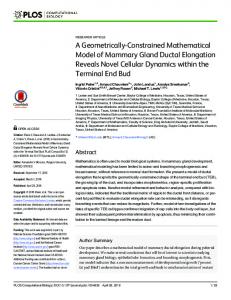
• The damage gradient appears only in the failure criterion and is energetically dissipative by nature, affecting distribution and evolution of the damage field. It is thus physically consistent with the motivation of accounting for microscopic nonlocal interactions. • The material behavior during the failure process is fully determined by two constitutive functions. In particular, the optimal ones allow defining an equivalent cohesive zone model of general softening laws, with the parameters calibrated from standard material properties. • The incorporated length scale can be regarded either as a numerical parameter or a material property. For the former, it has negligible, if not no, effects on the numerical results, so long as the sharp crack topology and the damage field of high gradient are well resolved. • The conjugate driving force vanishes as the damage approaches to unity. Consequently, the localization bandwidth tends to a finite limit value, not exhibiting spurious widening. This property is indispensable for modeling localized failure in quasi-brittle solids. The remainder of this paper is structured as follows. Section 2 addresses the constitutive relations and damage evolution law of the proposed gradient-damage model within the standard framework of thermodynamics, together with the governing equations in strong and weak forms. In Section 3 the constitutive functions optimal for quasi-brittle failure in solids are postulated, with the involved parameters calibrated for those frequently adopted softening laws. Section 4 is devoted to the multi-field finite element implementation and solution algorithm of the proposed model. Numerical performances of the proposed model are investigated in Section 5, regarding several benchmark tests of concrete under mode-I and mixed-mode failure. The most relevant conclusions are drawn in Section 6. Finally, Appendix compares the proposed gradient-damage model to other similar ones, closing this paper. Notation. Compact tensor notation is used in this paper as far as possible. As a general rule, scalars are denoted by italic light-face Greek or Latin letters (e.g. a or λ); vectors, second- and fourth-order tensors are signified by italic boldface minuscule, majuscule letters and blackboard-bold majuscule characters like a, A and A, respectively. The inner products with single and double contractions are denoted by ‘·’ and ‘:’, respectively. 2. Theoretical aspect As shown in Fig. 1, let Ω ⊂ Rn dim (n dim = 1, 2, 3) be the reference configuration of a solid subjected to distributed body forces b∗ . The solid is kinematically characterized by the displacement field u(x) and (infinitesimal) strain field ϵ(x) := ∇ sym u(x), for the symmetric gradient operator ∇ sym (·) with respect to the spatial coordinate x. The external boundary ∂Ω ⊂ Rn dim −1 , with the outward unit normal denoted by vector n, is split into two disjointed parts ∂Ωu and ∂Ωt , i.e., ∂Ωu ∩ ∂Ωt = ∅ and ∂Ωu ∪ ∂Ωt = ∂Ω , on which given displacements u∗ (x) for x ∈ ∂Ωu and tractions t∗ (x) for x ∈ ∂Ωt are applied, respectively. 2.1. Constitutive relations For any admissible deformation process, the first and second laws of thermodynamics in global form give the following non-negative energy dissipation rate D˙ ∫ ( ) ˙ σ : ϵ˙ − ψ˙ dV ≥ 0 (2.1) D= Ω

where σ is the stress tensor conjugate to the infinitesimal strain ϵ, with (˙) being the time derivative; ψ represents the local free energy density potential of the solid. For an isotropic damaging solid, the local free energy density potential ψ is expressed as the following general form ψ(ϵ, d) = ω(d)ψ0 (ϵ)

(2.2)

with the (monotonically decreasing) energetic degradation function ω(d) in terms of a single damage variable d ∈ [0, 1]. For hyperelastic materials, the initial strain energy density ψ0 reads ψ0 (ϵ) =

1 1 ϵ : E0 : ϵ = σ¯ : C0 : σ¯ 2 2

(2.3)

616

J.-Y. Wu / Comput. Methods Appl. Mech. Engrg. 328 (2018) 612–637

Fig. 1. Problem setting of a cracking solid medium.

where the effective stress tensor σ¯ is defined by the linear elastic relations σ¯ = E0 : ϵ,

ϵ = C0 : σ¯

(2.4)

for the material elastic stiffness E0 and compliance C0 , respectively. With the above local free energy density potential, the thermodynamic laws (2.1) become ∫ ( ∫ ( ∂ψ ) ∂ψ ) ˙ ˙ D= σ− : ϵ˙ dV + − d dV ≥ 0 (2.5) ∂ϵ ∂d Ω B where B ⊆ Ω denotes the localization band in which damage lumps, with the exterior domain Ω \ B free of damage. As the strain rate ϵ˙ is arbitrary and the damage rate d˙ ≥ 0 is non-negative, standard arguments [61] yield ∂ψ σ = = ω(d)σ¯ = ω(d)E0 : ϵ (2.6) ∂ϵ together with the following energy dissipation rate ∫ ∂ψ D˙ = Y d˙ dV ≥ 0, Y := − = −ω′ (d)Y (2.7) ∂d B where the damage energy release rate (driving force) Y is conjugate to the damage variable d, expressed in terms of the first derivative ω′ (d) = ∂ω/∂d and the reference value Y as ∂ψ 1 1 Y= = ψ0 (ϵ) = ϵ : E0 : ϵ = σ¯ : C0 : σ¯ . (2.8) ∂ω 2 2 The above isotropic constitutive relations do not discriminate non-symmetric material behavior in tension and compression; see Remark 2.1 for a simple remedy. Remark 2.1. To characterize the non-symmetric tensile and compressive material behavior, a modified reference energy Y is introduced as [52] √ ) 1 2 1 ( Y= σ¯ eq , σ¯ eq = βc ⟨σ¯ 1 ⟩ + 3 J¯2 (2.9) 2E 0 1 + βc

J.-Y. Wu / Comput. Methods Appl. Mech. Engrg. 328 (2018) 612–637

617

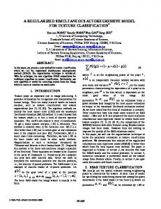
Fig. 2. 2-D failure envelope of normal concrete under dominant tension.

where E 0 is Young’s modulus of the material; σ¯ 1 and J¯2 := 12 s : s denote the first major principle value of the effective stress tensor σ¯ and the second invariant of the deviatoric one s¯ = σ¯ − (tr σ¯ )1/3, respectively; Macaulay brackets ⟨·⟩ are defined as ⟨x⟩ = max(x, 0). The material parameter βc := f c / f t − 1 is related to the ratio between the uniaxial compressive strength f c and tensile one f t . For normal concrete, the value f c / f t = 10 generally applies. The classical Rankine criterion is recovered for β → ∞. With the above re-definition, the failure envelope of concrete in dominant tension can be well captured as shown in Fig. 2. □ 2.2. Damage evolution law Once a specific failure criterion is fulfilled, in the solid Ω a sharp crack S ⊂ Rn dim −1 with the unit normal vector nS is initiated as in Fig. 1. In accordance with Griffith’s fracture mechanics, the energy dissipation rate is proportional to evolution of the crack surface area AS [4,65] ∫ D˙ = G f A˙ S ≥ 0, AS := dA (2.10) S

for the fracture energy G f per unit crack surface, usually regarded as a material property. Motivated by the phase-field theory [44,52], the sharp crack topology AS is regularized by a functional Ad (d) defined within the localization band B ⊆ Ω such that ∫ ∫ ∫ AS = dA = δS dV ≈ γ (d) dV = Ad (d) (2.11a) S

B

B

where the crack surface density function γ (d), approximating the Dirac-delta δS along the sharp crack S, is expressed in terms of the damage variable d and its spatial gradient ∇d which are not independent. Without loss of generality, the following generic crack surface density function is considered [52] ∫ 1√ ⏐ ⏐2 ] 1 [1 α(d) + b⏐∇d ⏐ with c0 = 4 α(β) dβ (2.11b) γ (d) = c0 b 0 where the crack geometric function α(d) characterizes homogeneous damage evolution; b is a length scale characterizing the localization band B; c0 > 0 is a scaling parameter such that the sharp crack surface AS is recovered

618

J.-Y. Wu / Comput. Methods Appl. Mech. Engrg. 328 (2018) 612–637

for a fully softened crack. Note that the regularized functional (2.11) is introduced in a rigorous geometric context, extending the classical framework established by Miehe et al. [66]. The energy dissipation rates (2.7) and (2.10) characterize evolution of the regularized crack and the sharp counterpart, respectively. Accordingly, the following energetic equivalence holds D˙ =

∫

Y d˙ dV = B

∫

G f γ˙ (d) dV

B

= G f A˙ S

(2.12a)

or, equivalently, ∫ ∫ ( ) RD dV = −Y d˙ + G f γ˙ dV = 0 B

(2.12b)

B

for the difference RD := −Y d˙ + G f γ˙ of the energy dissipation rates given by the local and nonlocal (gradient) damage evolution. As can be seen from Appendix, the so-called insulation condition on the nonlocal energy residual [64] is nothing but the natural outcome of the energetic equivalence together with the geometric regularization of the sharp crack topology. Application of the divergence theorem then yields ∫ ∫ ∫ ( ) ( ) 2 ˙ RD dV = −Y + G f δd γ d dV + bG f ∇d · nB d˙ dA = 0 (2.13) c 0 B B ∂B where nB is the outward unit normal vector of the boundary ∂B; the variational derivative δd γ of the crack surface density functional (2.11b) is expressed as ] [ ( ) 1 1 ′ α (d) − 2b∆d (2.14) δd γ := ∂d γ − ∇ · ∂∇d γ = c0 b for the Laplacian ∆d = ∇ · ∇d and the first derivative α ′ (d) := ∂α/∂d. Calling for the dissipative nature of damage evolution, the energetic equivalence (2.12) or (2.13) yields the Kuhn– Tucker loading/unloading conditions d˙ ≥ 0,

˙ dg(Y, d) ≡ 0

g(Y, d) ≤ 0,

in B

(2.15a)

or, equivalently, g(Y, d) := Y − G f δd γ

{

=0 0 d˙ = 0.

(2.15b)

Furthermore, the boundary condition of Neumann-type supplements ∇d · nB = 0

on ∂B.

(2.16)

Compared to the classical local damage model or the gradient-enhanced counterpart, the failure criterion (2.15) is not constructed ad hoc, but rather emerges rigorously from the geometric regularization and energetic equivalence. With the presence of Laplacian ∆d, well-posedness of the resulting (initial) boundary value problem is guaranteed. Note that rate-dependent materials can also be considered; see [52] for the details. Remark 2.2. In derivation of the above damage evolution law of gradient-type, the standard framework of thermodynamics is used with no extra assumption. Moreover, the damage gradient appears only in the energy dissipation rate and the resulting failure criterion, but not in the Helmholtz free energy density potential. Namely, its energetic contribution is fully dissipative. This fact is consistent with the physical motivation of microscopic nonlocal interactions; see Appendix for the comparison with the existing gradient-damage models. In the literature, Planas et al. [67]; Mazars and Pijaudier-Cabot [65] employed similar concepts to investigate the relationship between fracture mechanics and nonlocal damage models, but none of them derived the above damage evolution law. □

619

J.-Y. Wu / Comput. Methods Appl. Mech. Engrg. 328 (2018) 612–637

2.3. Governing equations With the above constitutive relations and damage evolution law, the governing equations for the solid Ω are then expressed as { ∇ · σ + b∗ = 0 in Ω (2.17) Y − G f δd γ = 0 ∀d˙ > 0 in B supplemented by the following boundary conditions of Neumann-type { σ · n = t∗ on ∂Ωt ∇d · nB = 0 on ∂B.

(2.18)

In the strong form (2.17), the first one is the conventional equilibrium equation and the second one governs the damage evolution law upon damage loading. Let us introduce the following test and trial spaces { ⏐ } { ⏐ } Uu := u⏐u(x) = u∗ ∀x ∈ ∂Ωu , Vu := δu⏐δu(x) = 0 ∀x ∈ ∂Ωu (2.19a) } { ⏐ } { ⏐ ˙ ≥ 0 ∀x ∈ B , Ud := d ⏐d(x) ∈ [0, 1], d(x) Vd := δd ⏐δd(x) ≥ 0 ∀x ∈ B . (2.19b) In accordance with the weighted residual method, the governing equations (2.17) and boundary conditions (2.18) can be rewritten as the following weak form: Find u ∈ Uu and d ∈ Ud such that ⎧∫ ⎪ sym ⎪ ∀δu ∈ Vu ⎨ σ : ∇ δu dV = δP Ω ∫ (2.20) ( ) ⎪ ⎪ ⎩ −Y δd + G f δγ dV = 0 ∀δd ∈ Vd B

for the virtual power δP of external forces and the variation δγ of the crack surface density function ∫ ∫ δP = b∗ · δu dV + t∗ · δu dA Ω ∂Ωt [ ] 1 1 ′ δγ = α (d) δd + 2b∇d · ∇δd c0 b

(2.21a) (2.21b)

where the divergence theorem has been considered. Note that in the numerical implementation it is not necessary to explicitly impose the natural boundary conditions (2.18) of Neumann-type, but rather, they are intrinsically accounted for in the weak form (2.20); see Section 4 for details. Remark 2.3. Pre-defined cracks S can be accounted for either by the Dirichlet condition d(x) = 1 for x ∈ S or directly by the mesh discretization; see [68]. In this work, the later strategy is adopted. □ Remark 2.4. The proposed gradient-damage model is equivalent to the following variational formulation ) (∫ ∫ ∫ ∫ ∗ ∗ δΠ = 0 with Π = ψ(ϵ, d) dV + G f γ (d) dV − b · u dV + t · u dA Ω

B

Ω

(2.22)

∂Ωt

which is a regularized counterpart to the variational approach to fracture [39] and the free discontinuity problem [69]. That is, the damage evolution minimizes the total energy of the solid under an irreversibility condition preventing self-healing of cracks; see [41] for more details. □ 3. Optimal constitutive functions As in the PFM [44], the proposed gradient-damage model is also characterized by two constitutive functions, i.e., the energetic degradation function defining the free energy density potential and the crack geometric function regularizing the sharp crack topology. In this work, the optimal constitutive functions, recently proposed in [52] for quasi-brittle failure in solids, are employed.

620

J.-Y. Wu / Comput. Methods Appl. Mech. Engrg. 328 (2018) 612–637

3.1. Energetic degradation function The energetic degradation function ω(d) ∈ [0, 1] satisfies the following properties [44] ω′ (d) < 0

and

ω(0) = 1,

ω(1) = 0,

ω′ (1) = 0.

Motivated by the analysis presented in [60], we suggest adopting the following generic form ( )p 1−d , Q(d) = a1 d + a1 a2 d 2 + a1 a2 a3 d 3 + · · · ω(d) = ( )p 1 − d + Q(d)

(3.1)

(3.2)

for the exponent p ≥ 1 and model parameters ai (i = 1, 2, 3, . . .) to be determined later. Though higher-order polynomials or other types of functions can also be considered, the strictly positive function Q(d) > 0 is here postulated as a cubic polynomial, i.e., i = 1, 2, 3. Remark 3.1. The energetic degradation function (3.2) recovers some particular examples adopted in the literature ⎧( )p ( )p Q(d) = 1 − 1 − d ⎪ ⎨ 1( − d ) p ( )q ( )q (3.3) ω(d) = 1−d ⎪ Q(d) = 1 + m 0 d − 1 − d )q ⎩( 1 + m0d for the exponent q and positive parameter m 0 > 0. The first power function, with p = 1 and p = 2, respectively, has been widely adopted in the local damage models [70] and in the phased-field models for brittle fracture [41]. The second function with p = q = 2 was employed in the gradient-damage model proposed by Lorentz and Godard [60]. □ 3.2. Crack geometric function Though not necessarily, it is generally assumed that the geometric function α(d) satisfies the following properties α(0) = 0,

α(1) = 1.

Without loss of generality, the following quadratic polynomial can be considered [52] ( ) α(d) = ξ d + 1 − ξ d 2 ∈ [0, 1] ∀d ∈ [0, 1]

(3.4)

(3.5)

for the non-negative parameter ξ ∈ [0, 2]. For brittle fracture, the quadratic one with ξ = 0 [40,44,71] and the linear one with ξ = 1 [46,55] have been dominantly adopted in the literature, resulting in an infinite localization bandwidth Du = +∞ and a finite one Du = 2b, respectively. In this work, the crack geometric function (3.5) with ξ = 2 is adopted, i.e., ∫ 1√ ∫ 1 1 π 2 α(d) = 2d − d H⇒ c0 = 4 α(β) dβ = π, Du = b dβ = b. (3.6) √ 2 α(β) 0 0 This crack geometric function is optimal for those softening laws frequently adopted for quasi-brittle failure, since it automatically guarantees bounded growth of the localization band and eases satisfaction of the irreversibility condition of cracking evolution; see [52] for more details. Remark 3.2. As shown in Fig. 3, with the geometric function (3.6) a sharp crack is regularized by the crack surface density function (2.11b) into the following damage profile [52] ∫ 1 ( |x | ) 1 n |xn | = b dβ H⇒ d(x) = 1 − sin (3.7) √ b α(β) d ( ) for the signed distance xn := x − xS · nS ∈ [−Du , Du ] between point x and the closest point xS on the sharp crack surface S. Note that the sharp crack topology is recovered for a vanishing length scale b → 0. In 2-D cases, the Γ -limit Ad → AS = 0.5 for the crack surface functional (2.11) is shown in Fig. 4, regarding a unit square plate with an edge crack. As the length scale b decreases below a certain threshold, the sharp crack topology AS can be approximated by the regularized one Ad with sufficient precision. □

J.-Y. Wu / Comput. Methods Appl. Mech. Engrg. 328 (2018) 612–637

621

Fig. 3. Ultimate damage profile d(x) in 1-D case governed by the crack geometric function α(d) = 2d − d 2 .

(a) Ad = 0.5220 for b = 0.05.

(b) Ad = 0.5090 for b = 0.02.

(c) Ad = 0.5047 for b = 0.01.

(d) Ad = 0.5031 for b = 0.005.

Fig. 4. Γ -convergence of a unit square plate with an edge crack [52]: Regularized crack surface Ad (d) governed by the crack geometric function α(d) = 2d − d 2 for different length scales b and a fixed mesh size h = 0.001. The sequence of pictures visualizes the Γ -limit Ad → AS = 0.5 of the crack surface functional (2.11). Note the finite support of the resulting localization band in all cases.

622

J.-Y. Wu / Comput. Methods Appl. Mech. Engrg. 328 (2018) 612–637

(a) Softening curves given by the proposed gradient-damage model.

(b) Softening curves frequently adopted for quasi-brittle solids.

Fig. 5. Softening laws predicted by the proposed gradient-damage model and those frequently adopted for quasi-brittle solids.

3.3. Model parameters

For the energetic degradation function (3.2) and crack geometric function (3.6), in 1-D case the stress σ and apparent displacement jump w across the localization band B are analytically given by [52] √( )( )p 2 − d∗ 1 − d∗ ∗ (3.8a) σ (d ) = f t 2P ∗ √ ] 1 √ ∫ ∗[ 4 2G f d 2−β P(β) − 2 β · P(β) P∗ ∗ w(d ) = −( (3.8b) ( )p · )p ( ) p dβ π ft 2 − d∗ 1 − d∗ 1−β 1−β 0 for the failure strength f t and polynomial function P(d) √ E0 G f ft = 2 , P(d) = 1 + a2 d + a2 a3 d 2 + · · · π · ba1

(3.9)

where the value P ∗ := P(d ∗ ) is evaluated with respect to the maximum damage d ∗ attained at the sharp crack surface S. As shown in Fig. 5(a), the relations (3.8) define a general softening law independent of the length scale b, while those frequently adopted ones for quasi-brittle failure are depicted in Fig. 5(b). After some tedious but straightforward mathematic manipulations, the initial slope k0 < 0 of the softening curve σ (w) and the ultimate crack opening wc > 0 with vanishing stress are expressed as ) ]3/2 ∂σ 1 f t2 [ ( =− 2 a2 + p + 1 d →0 ∂w 16 G f ( )1− p/2 2G f √ wc : = lim w= 2P(1) lim 1 − d∗ . d ∗ →1 d ∗ →1 ft k0 : = lim ∗

(3.10a) (3.10b)

Consequently, the exponent p = 2 renders a positive apparent displacement jump wc ∈ (0, +∞) across the localization band B and p > 2 yields an infinite value wc = +∞, while the exponent p < 2 gives a vanishing one wc = 0 which is not appropriate for quasi-brittle solids. Therefore, only the exponent p ≥ 2 is considered hereafter.

J.-Y. Wu / Comput. Methods Appl. Mech. Engrg. 328 (2018) 612–637

623

For the cubic polynomial Q(d) in the energetic degradation function (3.2), the coefficients ai (i = 1, 2, 3) are determined as ( ) 1) 4 E0 G f G f 2/3 ( , a = 2 −2k − p+ (3.11a) a1 = 2 0 2 2 πb f t 2 ft ⎧ p>2 ⎨0 [ ] ) a 3 = 1 1 ( wc f t )2 ( (3.11b) ⎩ − 1 + a2 p=2 a2 8 G f for the failure strength f t > 0, initial modulus (slope) k0 < 0 and ultimate crack opening wc > 0 of a target softening curve σ (w) to be approximated. Once the length scale b is given or calibrated, the parameters a1 , a2 and a3 can thus be determined from the standard material properties (i.e., Young’s modulus E 0 , failure strength f t , fracture energy G f ) and the target softening curve. In particular, the following optimal parameters are calibrated for those softening laws frequently adopted for quasi-brittle failure in solids [52]: • Linear softening curve: p = 2, a2 = − 21 and a3 = 0 ( ) ft f2 σ (w) = f t max 1 − w, 0 , k0 = − t , 2G f 2G f

wc =

2G f ft

• Exponential softening curve: p = 25 , a2 = 25/3 − 3 and a3 = 0 ( f ) f2 t σ (w) = f t exp − w , k0 = − t , wc = +∞ Gf Gf • Hyperbolic softening curve: p = 4, a2 = 27/3 − 4.5 and a3 = 0. ( f t )−2 2f2 σ (w) = f t 1 + w , k0 = − t , wc = +∞ Gf Gf • Cornelissen et al. [72] softening curve for normal concrete: p = 2, a2 = 1.3868 and a3 = 0.6567 [( ) ( ) ( ) ( )] σ (w) = f t 1.0 + η13r 3 exp −η2r − r 1.0 + η13 exp −η2 Gf f t2 , wc = 5.1361 Gf ft for the normalized crack opening r := w/wc as well as the parameters η1 = 3.0 and η2 = 6.93. k0 = −1.3546

(3.12)

(3.13)

(3.14)

(3.15a) (3.15b)

The resulting softening curves (3.8) are compared in Fig. 6 against the target ones. Among them, the linear softening curve is exactly reproduced, while the discrepancies for the exponential and hyperbolic ones are invisible. For the Cornelissen et al. [72] softening curve, the observed discrepancy is also very satisfactory, though only the cubic polynomial Q(d) is considered in the energetic degradation function (3.2). Increasing the order of Q(d) or using other functions may reduce the discrepancy. Other softening laws can be similarly considered. 4. Numerical implementation In this section, the weak form (2.20) of the proposed model is numerically implemented in the multi-field FEM. Note again that the natural boundary conditions (2.18) of Neumann-type are intrinsically accounted for. 4.1. Finite element discretization The computational domain Ω is discretized by the triangulation T h , consisting of n e elements and n p element nodes. The super-index h indicates a typical mesh size based on the finite element domain T h . As mesh induced anisotropic effects may favor some particular damage orientations and result in an over-evaluation of the fracture energy [73], for 2-D problems either unstructured triangular piecewise linear element [55] or structured quadrilateral bilinear one [60,74] is preferred in the discretization. In this case, each element node has three nodal degrees of freedom (dofs): two for the displacement field and one for the damage field. Different from the classical

624

J.-Y. Wu / Comput. Methods Appl. Mech. Engrg. 328 (2018) 612–637

(a) Linear softening law.

(b) Exponential softening law.

(c) Hyperbolic softening law.

(d) Cornelissen’s softening law.

Fig. 6. General softening curves predicted from the proposed gradient-damage model with optimal constitutive functions ( f t = 3.0 MPa, G f = 0.12 N/mm).

nonlocal and gradient-enhanced damage models, the damage field is here treated as a nodal variable and its continuity is automatically guaranteed. Moreover, in order to render mesh independent numerical results, the finite element mesh has to be uniform and fine enough around the localization band. On the one hand, non-uniform mesh induces artificial inhomogeneities and favors nucleation of cracks (in the sense of damage localization) in refined zones. On the other ) it is necessary ( hand, 1 for the element size h be much smaller than the localization bandwidth 2D = π b, i.e., h ≤ 15 ∼ 10 b, such that the precision of the fracture energy can be guaranteed in the discrete context [41]. In accordance with the FEM, the field uh and the resulting strain field ϵ h are approximated in terms { }displacement T of the nodal displacements χ := χ i uh (x) =

np ∑ i=1

Ni (x)χ i = N(x)χ ,

ϵ h (x) =

np ∑

Bi (x)χ i = B(x)χ

(4.1)

i=1

where in 2-D cases, the interpolation matrix N(x) and displacement–strain matrix B(x) have the components ⎡ ⎤ [ ] ∂ x Ni 0 Ni (x) 0 ∂ y Ni ⎦ Ni (x) = , Bi = ⎣ 0 0 Ni (x) ∂ y Ni ∂ x Ni for the interpolation function Ni (x) associated with the element node i.

(4.2)

J.-Y. Wu / Comput. Methods Appl. Mech. Engrg. 328 (2018) 612–637

625

h h Similarly, { }T the damage field d and its gradient ∇d are approximated in terms of the nodal damage variables χ˜ := χ˜ i

d h (x) =

np ∑

˜ χ˜ , N˜ i (x)χ˜ i = N(x)

∇d h (x) =

i=1

np ∑

˜ i (x)χ˜ = B(x) ˜ χ˜ B

(4.3)

i=1

for the corresponding interpolation matrices of the following components [ ] ∂ x Ni ˜ ˜ Ni (x) = Ni (x), Bi = ∂ y Ni

(4.4)

associated with the node i of elements within the localization band B. Note that, though not necessarily, identical interpolation functions Ni (x) are generally employed for both the displacement and damage fields. With the above finite element approximation, the weak form (2.20) results in the equilibrium equations in residual form ne ∫ R : = f ext − B T σ dV = 0 (4.5a)

A ∫ −A n=1 ne

˜ : = ˜f ext R

n=1

Ωe

Be

[

) ] ( ˜ T ω′ Y + 1 1 N ˜ T α ′ + 2b B ˜ T ∇d G f dV = 0 N c0 b

(4.5b)

where A represents the standard assembly operator; the external force vectors fext and f˜ext are expressed as ne

f ext =

(∫

A n=1

Ωe

N T b∗ dV +

∫ ∂Ωt,e

) N T t ∗ dS ,

˜f ext = 0

(4.6)

Note that in the numerical implementation the localization band B h ⊆ Ω h can be coincident with the whole computational domain Ω h . Alternatively, a smaller sub-domain can be taken, so long as it encompasses the potential crack path determined a priori. This property is useful in the computational modeling of localized failure in solids. 4.2. Solution algorithm The system of nonlinear equations (4.5) in general are solved in the incremental context. That is, during the time interval [0, T ] of interest all the state variables are considered at the N discrete interval [tn , tn+1 ] for n = 0, 1, 2, . . . , N − 1. For a typical time increment [tn , tn+1 ] of size ∆t := tn+1 − tn , the system of nonlinear equations (4.5) is to be solved upon all state variables known at the instant tn . During each incremental step, either a monolithic or staggered algorithm can be employed to solve the unknowns; see [44] among many others. In the former one, the discrete governing equations (4.5) are linearized with respect to the nodal displacements and damage variables simultaneously, such that both unknowns are solved by, e.g., a Newton-type method. If such a monolithic algorithm works, the final solution converges rapidly. However, the monolithic algorithm is in general not robust enough [47]. To this end, the discrete governing equations (4.5) are frequently solved by fixing the damage field d or the displacement field u alternatively, resulting in the staggered algorithm with nevertheless, rather slow convergence rate. More recently, Farrell and Maurini [75] interpreted the staggered algorithm as a nonlinear Gauss–Seidel scheme and used the over-relaxed strategy to accelerate the iteration, greatly increasing the computational efficiency. Furthermore, once the iterative solution is reached within the convergence basin (e.g., the relative L 2 -norm of the residual is less than a given tolerance, say, 10−3 ), the over-relaxed staggered algorithm is switched to a Newtontype scheme, e.g., an active-set Newton method with backtracking line search, until the final solution converges. Accordingly, the robustness and monotonic convergence of the staggered algorithm are combined with the asymptotic quadratic convergence of the Newton method. In this work, the above composite over-relaxed staggered-monolith scheme is used, with the non-symmetric material behavior accounted for as in Remark 2.1.

626

J.-Y. Wu / Comput. Methods Appl. Mech. Engrg. 328 (2018) 612–637

Fig. 7. Mode-I failure of four-point bending notched beams reported in [76]: Geometry (unit of length: mm), loading and boundary conditions. Three different specimens of initial notch depths 10 mm, 30 mm and 50 mm are investigated.

5. Numerical results In all numerical examples presented in this section, unstructured piece-wise linear triangular elements are used to discretize the computation domain. In particular, sufficiently fine uniformly distributed unstructured triangular elements are used in the sub-domain surrounding potential crack paths, while those remaining regions are discretized using triangular elements of larger size. Note that this a priori h-adaptive mesh strategy is currently used only to reduce the computational cost, not being a limitation of the proposed model. For all cases, plane stress state is assumed, and the Cornelissen et al. [72] softening law is employed, resulting in the model parameters p = 2, a2 = 1.3868 and a3 = 0.6567. 5.1. Mode-I failure of notched beams Let us consider the test of four-point bending concrete notched beams reported in [76]. The specimen, depicted in Fig. 7, is of dimensions 500 ×100 ×50 mm3 and simply supported with a span 450 mm. A vertical notch of width 5 mm was pre-fabricated at the bottom center of the specimen. Three different notch depths, i.e., 10 mm, 30 mm and 50 mm, respectively, were investigated in the test. The vertically downward loads F ∗ were applied at two points trisecting the span via displacement control, with the deflection u ∗ at the notch bottom monitored. For all specimens, a vertical (mode-I) crack initiates at the notch tip and propagates upward to the beam top until the eventual failure occurs. The material properties are taken from [76], i.e., Young’s modulus E 0 = 3.8 × 104 MPa, Poisson’s ratio ν0 = 0.2, tensile strength f t = 3.0 MPa and fracture energy G f = 0.125 N/mm. The effect of mesh size h is discussed with respect to the specimen with an initial notch depth 30 mm. For the length scales b = 5.0 mm and b = 2.5 mm, respectively, two different mesh sizes, i.e., a coarse one with h = 0.25 mm and a fine one with h = 0.125 mm, are considered. The numerical damage profiles at the deflection u ∗ = 0.7 mm are illustrated in Fig. 8. As the damage profiles given from two mesh sizes almost coincide, only the ones for h = 0.125 mm are presented. Furthermore, though the localization bandwidth is proportional to the length scale b, the (mode-I) failure mode is not affected. The numerical results of load versus deflection are shown in Fig. 9. For an identical length scale b, the mesh size h affects neither the damage profile nor the global response. Namely, the proposed model is mesh-size dependent. The influence of length scale b is first investigated regarding the specimen with an initial notch depth 30 mm. Five length scales, b = 2.5 mm, 5.0 mm, 10.0 mm, 15.0 mm and 20.0 mm, respectively, are considered, with the mesh size fixed as h = 0.25 in all cases. It can be seen from the numerical curves of load F ∗ versus deflection u ∗ shown in Fig. 10 that, the global responses converge for the length b ≤ 5.0 mm. This implies that the sharp crack topology AS is approximated by the regularized one Ad with sufficient precision for the length scale b ≤ 5.0 mm. It is also validated that the proposed model with the optimal constitutive functions (3.2) and (3.6) is equivalent to the cohesive zone model (3.8) with no extrinsic length scale. The effect of length scale b is then investigated regarding all specimens with various initial notch depths. Two different length scales, i.e., b = 5.0 mm and b = 2.5 mm, are considered for a fixed mesh size h = 0.25 mm. The

J.-Y. Wu / Comput. Methods Appl. Mech. Engrg. 328 (2018) 612–637

627

(a) Internal length scale b = 5.0 mm.

(b) Internal length scale b = 2.5 mm. Fig. 8. Mode-I failure of a notched beam (notch depth: 30 mm) subjected to fourth-point bending: damage profiles with respect to the length scale b. The damage profile is almost irrelevant to mesh size h and only the ones for h = 0.125 mm are presented.

(a) Internal length scale b = 2.5 mm.

(b) Internal length scale b = 5.0 mm.

Fig. 9. Mode-I failure of notched beams (notch depth: 30 mm) subjected to fourth-point bending: Curves of applied load versus central deflection with respect to the mesh size h within the localization band. Two mesh sizes, i.e., h = 0.25 mm and h = 0.125 mm, are considered.

numerical curves of load F ∗ versus deflection u ∗ are depicted in Fig. 11. The peak loads and softening regimes match the experimental results rather well, though the peak load for the notch depth 10 mm is somewhat over-evaluated similarly to the numerical result given from the discrete crack model [76]. Again, the global responses are almost independent of the length scale b ≤ 5 mm, so long as the sharp crack topology and the damage field of high gradient

628

J.-Y. Wu / Comput. Methods Appl. Mech. Engrg. 328 (2018) 612–637

Fig. 10. Mode-I failure of notched beams (notch depth: 30 mm) subjected to fourth-point bending: Curves of applied load versus central deflection with respect to different length scales b and a fixed mesh size h = 0.25 mm. The global responses converge as the length scale decreases below b ≤ 5 mm.

within the localization band are well resolved with sufficient precision. The same conclusions were also obtained in [52] for the uniaxial traction and three-point bending tests. The above results are rather distinct from the existing phase-field and gradient-damage models. On the one hand, for the existing phase-field models [43,44] the global responses depend heavily on the length scale b and only for the vanishing one b → 0 can the solution eventually converge [51]. Consequently, very small mesh 1 size, i.e., h ≤ ( 15 ∼ 10 )b, has to be used to resolve the highly non-uniform damage field within the localization band, resulting in an almost prohibitive computational cost. On the other hand, in the existing gradient-damage models [55,77] the length scale b is regarded as a physical or material property related to the microscopic structures of the solid. In this case, the length scale b is in general large, e.g., about (3 ∼ 8)da for normal concrete (where da is the maximum size of aggregates), yielding non-negligible errors between the regularized crack surface Ad and the sharp one AS ; see Fig. 4 for the illustration. As the energetic equivalence (2.12) no longer holds in this case, the length scale will affect the global responses and the structural size effect, manifested by over-estimations of the peak load and energy dissipation during the failure process [77]. Similar phenomena are also observed in the classical non-local (gradient-enhanced) damage models [4]. Comparatively, the proposed model, with the incorporated length scale regarded as a small but finite numerical parameter, resembles the cohesive zone model with no extrinsic length scale, avoiding the aforesaid deficiencies. Note that this choice does not preclude the possibility of regarding the length scale as a material property, which is, however, beyond the scope of this work and will be addressed elsewhere. 5.2. Mixed-mode failure of a L-shaped panel Next, let us consider the mixed-mode failure test of a L-shaped panel conducted by Winkler [78]. The geometry, loading and boundary conditions of the specimen are shown in Fig. 12. The bottom edge of the specimen is fixed. A vertical point load F ∗ is applied upward at a distance of 30 mm to the right edge of the horizontal leg, with the corresponding vertical displacement u ∗ at the same place recorded. Note that the widely adopted failure criterion based on average stress gives spurious crack path with large noisy oscillation and random changes [79], the linear fracture mechanics criterion in general has to be considered [80]. In the numerical simulation, the material properties are taken from the reference [78]: Young’s modulus E 0 = 2.585 × 104 MPa, Poisson’s ratio ν0 = 0.18, failure strength f t = 2.7 MPa, fracture energy G f = 0.09 N/mm. Three different mesh sizes, i.e., the coarse one with h = 1.0 mm, the medium one with h = 0.5 mm and the fine one with h = 0.25 mm, respectively, are used to discretize the computational domain. Two different length scales, i.e., b = 10 mm and b = 5 mm, respectively, are considered for all the mesh sizes. As shown in Figs. 13 and 14, the numerical damage profiles are rather smooth and agree well with the experimentally observed crack patterns, with no additional tracking strategy. As expected, on the one hand, the mesh

J.-Y. Wu / Comput. Methods Appl. Mech. Engrg. 328 (2018) 612–637

(a) Notch depth: 10 mm.

629

(b) Notch depth: 30 mm.

(c) Notch depth: 50 mm. Fig. 11. Mode-I failure of notched beams subjected to fourth-point bending: Curves of applied load versus central deflection with respect to different length scales b ≤ 5 mm and a fixed mesh size h = 0.25 mm.

Fig. 12. L-shaped panel [78]: Geometry, loading and boundary conditions (left; unit of length: mm); Crack paths (right).

630

J.-Y. Wu / Comput. Methods Appl. Mech. Engrg. 328 (2018) 612–637

(a) Coarse mesh (h = 1.0 mm).

(b) Medium mesh (h = 0.5 mm).

(c) Fine mesh (h = 0.25 mm).

Fig. 13. L-shaped panel: damage profiles for a fixed length scale b = 10 mm as the mesh size h decreases.

(a) Coarse mesh (h = 1.0 mm).

(b) Medium mesh (h = 0.5 mm).

(c) Fine mesh (h = 0.25 mm).

Fig. 14. L-shaped panel: damage profiles for a fixed length scale b = 5 mm as the mesh size h decreases.

size h has little effects on the numerical damage profile, and on the other hand, the length scale b does affect the localization bandwidth but not too much the damage profile. Figs. 15 and 16 compare the numerical curves of load F ∗ versus displacement u ∗ for various mesh sizes and length scales. As can be seen, the numerical prediction is independent of mesh size and length scale b ≤ 10 mm. Furthermore, though the initial stiffness of specimen is somewhat over-evaluated, all the numerical responses capture the experimental peak loads and softening regimes fairly well. Note that the above over-estimation is unavoidable for the given material properties and some modified ones have been suggested to match better the experimental data; see [80,81]. However, such data fitting is not performed here. 5.3. Mixed-mode failure of notched beams Finally, let us consider a series of notched beam tests subjected to mixed-mode failure reported in [82]. As depicted in Fig. 17, the specimen is of dimensions 675 ×150 ×50 mm3 , with a vertical notch of sizes 2 ×75 ×50 mm3 at the bottom center. In the first case, the stiffness at the upper left support is zero (i.e., three-point bending with

J.-Y. Wu / Comput. Methods Appl. Mech. Engrg. 328 (2018) 612–637

(a) Internal length b = 10 mm.

631

(b) Internal length b = 5 mm.

Fig. 15. L-shaped panel: Curves of load versus displacement for various mesh sizes.

(a) Coarse mesh h = 1.0 mm.

(b) Medium mesh h = 0.5 mm.

(c) Fine mesh h = 0.25 mm. Fig. 16. L-shaped panel: Curves of load versus displacement for various length scales.

K = 0), whereas in the second one it is infinite (i.e., four-point bending with K = ∞). The load F ∗ is applied under displacement control and the crack mouth opening displacement (CMOD) is monitored in both cases. In the numerical simulation, the material properties are taken from [82], i.e., Young’s modulus E 0 = 3.8×104 MPa, Poisson’s ratio ν0 = 0.2, tensile strength f t = 3.0 MPa and fracture energy G f = 0.069 N/mm. A single length scale b = 2.5 mm is considered, with two different mesh sizes, i.e., the coarse one with h = 0.5 mm and the fine one with

632

J.-Y. Wu / Comput. Methods Appl. Mech. Engrg. 328 (2018) 612–637

Fig. 17. Mixed-model failure test of notched beams [82]: Geometry (unit of length: mm), loading and boundary conditions.

Fig. 18. Mixed-model failure test of notched beams: Damage profiles. Left column (three-point bending): Experimental crack pattern (top); Numerical damage profile for b = 2.5 mm and h = 0.50 mm (middle); Numerical damage profile for b = 2.5 mm and h = 0.25 mm (bottom). Right column (four-point bending): Experimental crack pattern (top); Numerical damage profile for b = 2.5 mm and h = 0.50 mm (middle); Numerical damage profile for b = 2.5 mm and h = 0.25 mm (bottom).

h = 0.25 mm, respectively, used to discretize the computational domain. It is expected that the highly non-uniform damage field within the localization band can be well resolved. The numerical damage profiles for both three- and four-point bending tests are shown in Fig. 18. As expected, for both tests the mesh size has no effect on the predicted damage profiles which capture the experimental crack rather well. Specifically, regarding the support condition at the upper left, the crack emerges from the notch tip and propagates with different skew angles (with respect to the beam axis) to the beam top. The calculated curves of load versus crack mouth opening displacement (CMOD) are depicted in Fig. 19. Though the ratio b/ h varies, the numerical results obtained from both mesh sizes are very close to each other. For the threepoint bending test, not only the peak loads but also the softening regimes match the test results rather well. For the four-point one, the concordance of numerical results with the experimental evidence is clear until a sudden collapse occurs at about CMOD = 0.1 mm; see [83] for similar results.

J.-Y. Wu / Comput. Methods Appl. Mech. Engrg. 328 (2018) 612–637

(a) Three-point bending test (K = 0).

633

(b) Four-point bending test (K = ∞).

Fig. 19. Mixed-model failure test of notched beams: Curves of load versus CMOD.

6. Conclusions Motived by the unified phase-field theory [52], this work addresses a geometrically regularized gradient-damage model with energetic equivalence, bridging the damage and fracture mechanics for quasi-brittle failure in solids. The constitutive relations are derived consistently from the standard framework of thermodynamics, without introducing the extra insulation condition on the so-called nonlocal energy residual. With the sharp crack topology geometrically regularized as a localization band and the ensuing energetic equivalence between them, the damage evolution law of gradient-type and boundary condition of Neumann-type naturally emerge. Being fully energetically dissipative, the damage gradient physically accounts for the underlying microscopic nonlocal interactions. As the crack is implicitly represented by the damage and its gradient, the crack propagation is intrinsically tracked by the damage evolution law, such that tedious crack tracking strategies are entirely avoided. The material behavior during the failure process is completely defined by a bulk energetic function for the free energy potential and a geometric one for regularizing the sharp crack topology. Optimal constitutive functions are postulated for modeling localized failure in quasi-brittle solids, with the involved parameters determined from the target softening law of an equivalent cohesive zone model. The proposed gradient-damage model is numerically implemented into the multi-field finite element method and then applied to several benchmark tests of concrete under mode-I and mixed-mode failure. It is found that the incorporated length scale can be regarded either a numerical parameter or a material property. For the former, similarly to the cohesive zone model, the length scale has negligible, if not no, effects on the global responses, so long as the sharp crack topology and the damage field of high gradients within the localization band are well resolved. Furthermore, the localization bandwidth does not exhibit spurious damage growth, but approaches to a finite limit value scaled by the length scale. Numerical predictions, regarding the curve of load versus displacement and crack path, agree well with the experimental data, validating the proposed model for characterizing localized failure in quasi-brittle solids. Currently, the proposed gradient-damage model is limited only to infinitesimal deformations and quasi-static failure processes. A natural extension is to account for large deformations, particularly in dynamic situations. Permanent deformations and multi-physics problems with thermo-, hydro-, electro-, magneto-, etc., effects, can also be considered. Last but not least, the framework of multiscale (e.g., FE2 ) method or isogeometric analysis can be employed to improve the computational efficiency or numerical precision. All these relevant topics are on-going. Acknowledgments This work is supported by the National Natural Science Foundation of China (51678246) and the State Key Laboratory of Subtropical Building Science (2016KB12). Partial support from the Fundamental Research Funds for the Central University (2015ZZ078) and the Scientific/Technological Project of Guangzhou (201607020005) is also acknowledged.

634

J.-Y. Wu / Comput. Methods Appl. Mech. Engrg. 328 (2018) 612–637

Appendix. Comparison with other gradient-damage models In existing gradient-damage models [55–57,63], the free energy density functional ψ depends not only on the strain tensor ϵ and damage variable d, but also on the damage gradient ∇d 1 1 ω(d)ϵ : E0 : ϵ + E g ∇d · ∇d (A.1) 2 2 where the first term is the classical local free energy density potential; the second one characterizes microscopic nonlocal interactions in terms of the gradient parameter E g ≥ 0 to be determined. As the damage gradient appears in the free energy density potential, the standard framework of thermodynamics cannot be used straightforwardly. To overcome this issue, Polizzotto and Borino [62] introduced the so-called nonlocal energy residual and rewrote the local version of global Clausius–Duhem inequality (2.1) as ∫ D˙ loc = σ : ϵ˙ − ψ˙ + R ≥ 0 with R dV = 0 (A.2) ψ(ϵ, d, ∇d) =

B

where the nonlocal energy residual R accounts for microscopic interactions without modifying the classical constitutive relation (2.6) and damage driving force (2.7)2 . Accordingly, the local dissipation inequality reads D˙ loc = Y d˙ − E g ∇d · ∇ d˙ + R ≥ 0

(A.3a)

which implies independent evolution laws for the damage d and its gradient ∇d. To reconcile their in-between compatibility, Polizzotto and Borino [62] further introduced a non-local damage driving force Y¯ and wrote the energy dissipation rate as a bilinear form D˙ loc = Y¯ d˙ ≥ 0,

R = Y¯ · d˙ − Y d˙ + E g ∇d · ∇ d˙

leading to ∫ ∫ ∫ ( ) ¯ ˙ R dV = Y − Y − E g ∆d d dV + B

B

∂B

( ) E g ∇d · nB d˙ dA = 0

where integration by part has been considered. It then follows that { Y¯ = Y + E g ∆d ∀d˙ > 0 in B ∇d · nB = 0 on ∂B

(A.3b)

(A.4)

(A.5)

Moreover, a failure criterion has to be constructed a priori in order to determine the damage evolution law. For the local energy dissipation inequality (A.3b) in bilinear form, the damage criterion is heuristically motivated as g(Y¯ , κ) = Y¯ − κ(d) = Y + E g ∆d − κ(d) ≤ 0

(A.6)

for a damage threshold κ(d) to be determined. In existing gradient-damage models, the gradient parameter E g and damage threshold κ(d) are generally assumed ad hoc. Lorentz and Godard [60] first suggested determining them from 1-D closed-form solution. In particular, comparison of the damage criterion (A.6) to the one (2.15) gives Eg =

2G f 2 b , c0 b

κ(d) =

Gf ′ α (d) c0 b

(A.7)

both dependent on the fracture energy G f and length scale b. With the above gradient parameter E g and damage threshold κ(d), the resulting damage evolution law and governing equations are identical to those developed in this work. However, the second term in the free energy density potential (A.1), accounting for microscopic nonlocal interactions, is characterized by the damage parameter E g dependent on the fracture energy G f . Namely, it should be completely dissipative, but is assumed to be recoverable in existing models. Contrariwise, the aforesaid controversy does not arise in the proposed geometrically regularized gradient-damage model with energetic equivalence. Moreover, only standard thermodynamic arguments are considered, whereas it is unnecessary to introduce any extra assumption to reconcile compatibility between the damage d and its gradient ∇d.

J.-Y. Wu / Comput. Methods Appl. Mech. Engrg. 328 (2018) 612–637

635

References [1] [2] [3] [4] [5] [6] [7] [8] [9] [10] [11] [12] [13] [14] [15] [16] [17] [18] [19] [20] [21] [22] [23] [24] [25] [26] [27] [28] [29] [30] [31] [32] [33] [34] [35] [36] [37]

D. Ngo, A. Scordelis, Finite element analysis of reinforced concrete beams, ACI J. 64 (14) (1967) 152–163. Y. Rashid, Analysis of prestressed concrete pressure vessels, Nucl. Eng. Des. 7 (1968) 334–344. J. Rots, Computational Modeling of Concrete Fracture, Delft University of Technology, the Netherlands, 1988 (Ph.D. thesis). Z.P. Bažant, J. Planas, Fracture and Size Effects in Concrete and Other Quasi-Brittle Materials, CRC Press, New York, 1997. G. Pijaudier-Cabot, Z. Bažant, Nonlocal damage theory, J. Engng. Mech., ASCE 113 (1987) 1512–1533. R. Peerlings, R. de Borst, W. Brekelmans, J. de Vree, Gradient-enhanced damage for quasi-brittle materials, Internat. J. Numer. Methods Engrg. 39 (1996) 3391–3403. A. Krayania, G. Pijaudier-Cabotb, F. Dufour, Boundary effect on weight function in nonlocal damage model, Eng. Fract. Mech. 76 (14) (2009) 2217–2231. R. Peerlings, M. Geers, R. de Borst, W. Brekelmans, A critical comparison of nonlocal and gradient-enhanced softening continua, Internat. J. Solids Struct. 38 (2001) 7723–7746. M. Geers, R. de Borst, W. Brekelmans, R. Peerlings, Strain-based transient-gradient damage model for failure analyses, Comput. Methods Appl. Mech. Engrg. 160 (1998) 133–153. A. Simone, H. Askes, L. Sluys, Incorrect initiation and propagation of failure in non-local and gradient-enhanced media, Internat. J. Solids Struct. 41 (2004) 351–363. G. Di Luzio, B. Bažant, Spectral analysis of localization in nonlocal and over-nonlocal materials with softening plasticity and damage, Internat. J. Solids Struct. 42 (2005) 6071–6100. L. Poh, S. Swaddiwudhipong, Over-nonlocal gradient enhanced plastic-damage model for concrete, Internat. J. Solids Struct. 46 (2009) 4369–4378. C. Giry, F. Dufour, J. Mazars, Stress-based nonlocal damage model, Internat. J. Solids Struct. 48 (2011) 3431–3433. G. Nguyen, A damage model with evolving nonlocal interactions, Int. J. Solids Struct. 48 (2011) 1544–1559. G. Pijaudier-Cabot, K. Haidar, J. Dubé, Non-local damage model with evolving internal length, Int. J. Numer. Anal. Geomech. 28 (2004) 633–652. L. Poh, G. Sun, Localizing gradient damage model with decreasing interactions, Internat. J. Numer. Methods Engrg. (2016). http://dx.doi.org/ 10.1002/nme.5364. M. Jirásek, T. Zimmermann, Analysis of rotating crack model, J. Eng. Mech., ASCE 124 (8) (1998) 842–851. J. Simó, J. Oliver, F. Armero, An analysis of strong discontinuities induced by strain-softening in rate-independent inelastic solids, Comput. Mech. 12 (1993) 277–296. N. Moës, J. Dolbow, T. Belytschko, A finite element method for crack growth without remeshing, Internat. J. Numer. Methods Engrg. 46 (1999) 131–150. M. Jirásek, T. Belytschko, Computational resolution of strong discontinuities, in: H. Mang, F.R., Eberhardsteiner, J. Proceedings of the World Congress on Computational Mechanics (WCCM V), p. Available from: http://wccm.tuwien.ac.at, 2002. J.Y. Wu, Unified analysis of enriched finite elements for modeling cohesive cracks, Comput. Methods Appl. Mech. Engrg. 200 (45–46) (2011) 3031–3050. S. Loehnert, A stabilization technique for the regularization of nearly singular extended finite elements, Comput. Mech. 54 (2014) 523–533. A. Simone, Partition of unity-based discontinuous elements for interface phenomena: computational issues, Comm. Numer. Methods Engrg. 20 (2004) 465–478. G. Ventura, E. Benvenuti, Equivalent polynomials for quadrature in Heaviside function enriched elements, Internat. J. Numer. Methods Engrg. 102 (2015) 688–710. I. Babuška, U. Banerjee, Stable generalized finite element method (SGFEM), Comput. Methods Appl. Mech. Engrg. 201–204 (2012) 91–111. J.Y. Wu, F.B. Li, An improved stable XFEM (Is-XFEM) with a novel enrichment function for the computational modeling of cohesive cracks, Comput. Methods Appl. Mech. Engrg. 295 (2015) 77–107. E. Benvenuti, A regularized XFEM framework for embedded cohesive interfaces, Comput. Methods Appl. Mech. Engrg. 197 (49–50) (2008) 4367–4378. G. Ferté, P. Massin, N. Moë, 3d crack propagation with cohesive elements in the extended finite element method, Internat. J. Numer. Methods Engrg. 300 (2016) 347–374. F. Cazes, N. Moës, Comparison of a phase-field model and of a thick level set model for brittle and quasi-brittle fracture, Internat. J. Numer. Methods Engrg. 103 (2015) 114–143. N. Moës, C. Stolz, P.-E. Bernard, N. Chevaugeon, A level set based model for damage growth: The thick level set approach, Internat. J. Numer. Methods Engrg. 86 (2011) 358–380. P. Bernard, N. Moës, N. Chevaugeon, Damage growth modeling using the Thick Level Set (TLS) approach: Efficient discretization for quasi-static loadings, Comput. Methods Appl. Mech. Engrg. 233–236 (2012) 11–27. I. Aranson, V. Kalatsky, V. Vinokur, Continuum field description of crack propagation, Phys. Rev. Lett. 85 (2000) 118–121. A. Karma, D. a. Kessler, Phase-field model of mode III dynamic fracture, Phys. Rev. Lett. 87 (2001) 118–121. V. Hakim, A. Karma, Laws of crack motion and phase-field models of fracture, J. Mech. Phys. Solids 57 (2009) 342–368. R. Spatschek, E. Brener, A. Karma, Phase field modeling of crack propagation, Phil. Mag. 9 (2011) 75–95. R. Alicandro, A. Braides, J. Shah, Free-discontinuitiy problems via functionals involving the L 1 -norm of the gradient and their approximations, Interfaces Free Bound. 1 (1999) 17–37. L. Ambrosio, N. Fusco, D. Pallara, Functions of Bounded Variation and Free Discontinuity Problems, in: Oxf. Math. Monogr., The Clarendon Press, Oxford University Press, New York, 2000.

636

J.-Y. Wu / Comput. Methods Appl. Mech. Engrg. 328 (2018) 612–637

[38] A. Braides, G.D. Maso, A. Garroni, Variational formulation of softening phenomena in fracture mechanics: the one-dimensional case, Arch. Ration. Mech. Anal. 146 (1999) 23–58. [39] G. Francfort, J. Marigo, Revisting brittle fracture as an energy minimization problem, J. Mech. Phys. Solids 46 (8) (1998) 1319–1342. [40] B. Bourdin, G. Francfort, J.-J. Marigo, Numerical experiments in revisited brittle fracture, J. Mech. Phys. Solids 48 (4) (2000) 797–826. [41] B. Bourdin, G. Francfort, J.-J. Marigo, The Variational Approach to Fracture, Springer, Berlin, 2008. [42] H. Amor, J. Marigo, C. Maurini, Regularized formulation of the variational brittle fracture with unilateral contact: numerical experiments, J. Mech. Phys. Solids 57 (2009) 1209–1229. [43] C. Kuhn, R. Müller, A continuum phase field model for fracture, Eng. Fract. Mech. 77 (2010) 3625–3634. [44] C. Miehe, F. Welschinger, M. Hofacker, Thermodynamically consistent phase-field models of fracture: Variational principles and multi-field FE implementations, Internat. J. Numer. Methods Engrg. 83 (2010) 1273–1311. [45] M. Hofacker, C. Miehe, A phase field model of dynamic fracture: Robust field updates for the analysis of complex crack patterns, Internat. J. Numer. Methods Engrg. 93 (2013) 276–301. [46] B. Bourdin, J.-J. Marigo, C. Maurini, P. Sicsic, Morphogenesis and propagation of complex cracks induced by thermal shocks, Phys. Rev. Lett. 112 (2014) 014301. [47] M. Ambati, T. Gerasimov, L. de Lorenzis, A review on phase-field models for brittle fracture and a new fast hybrid formulation, Comput. Mech. 55 (2015) 383–405. [48] C.V. Verhoosel, R. de Borst, A phase-field model for cohesive fracture, Internat. J. Numer. Methods Engrg. 96 (2013) 43–62. [49] J. Vignollet, S. May, R. de Borst, C.V. Verhoosel, Phase-field model for brittle and cohesive fracture, Meccanica 49 (2014) 2587–2601. [50] S. Conti, M. Focardi, F. Iurlano, Phase field approximation of cohesive fracture models, Ann. Inst. Henri Poincare (C) Non Linear Anal. 33 (4) (2015) 1033–1067. [51] M. Focardi, F. Iurlano, Numerical insight of a variational smeared approach to cohesive fracture, J. Mech. Phys. Solids 98 (2017) 156–171. [52] J.Y. Wu, A unified phase-field theory for the mechanics of damage and quasi-brittle failure in solids, J. Mech. Phys. Solids 103 (2017) 72–99. [53] R. de Borst, C. Verhoosel, Gradient damage vs phase-field approaches for fracture: Similarities and differences, Comput. Methods Appl. Mech. Engrg. (2016). http://dx.doi.org/10.1016/j.cma.2016.05.015. [54] P. Sicsic, J. Marigo, From gradient damage laws to Griffith’s theory of crack propagation, J. Elasticity 113 (1) (2013) 55–74. [55] K. Pham, H. Amor, J.-J. Marigo, C. Maurini, Gradient damage models and their use to approximate brittle fracture, Int. J. Damage Mech. 20 (2011) 618–652. [56] M. Frémond, B. Nedjar, Damage, gradient of damage and principle of virtual power, Internat. J. Solids Struct. 33 (8) (1996) 1083–1103. [57] B. Nedjar, Elastoplastic-damage modelling including the gradient of damage: formulation and computational aspects, Int. J. Solids Struct. 38 (2001) 5421–5451. [58] G. Pijaudier-Cabot, N. Burlion, Damage and localisation in elastic materials with voids, Int. J. Mech. Cohesive Frictional Mater. 1 (1996) 129–144. [59] E. Lorentz, A. Andrieux, A variational formulation for nonlocal damage models, Int. J. Plast. 15 (1999) 119–138. [60] E. Lorentz, V. Godard, Gradient damage models: Towards full-scale computations, Comput. Methods Appl. Mech. Engrg. 200 (2011) 1927–1944. [61] B. Coleman, M. Gurtin, Thermodynamics with internal state variables, J. Chem. Phys. 47 (1967) 597–613. [62] C. Polizzotto, G. Borino, A thermodynamics-based formulation of gradient-dependent plasticity, Eur. J. Mech. A Solids 17 (1998) 741–761. [63] T. Liebe, P. Steinmann, A. Benallal, Theoretical and computational aspects of a thermodynamically consistent framework for geometrically linear gradient damage, Comput. Methods Appl. Mech. Engrg. 190 (2001) 6555–6576. [64] C. Polizzotto, Unified thermodynamic framework for nonlocal/gradient continuum theories, Eur. J. Mech. A Solids 22 (2003) 651–668. [65] J. Mazars, G. Pijaudier-Cabot, From damage to fracture mechanics and conversely: A combined approach, Internat. J. Solids Struct. 33 (20–22) (1996) 3327–3342. [66] C. Miehe, L. Schänzel, H. Ulmer, Phase field modeling of fracture in multi-physics problems. Part I. balance of crack surface and failure criteria for brittle crack propagation in thermo-elastic solids, Comput. Methods Appl. Mech. Engrg. 294 (2015) 449–485. [67] J. Planas, M. Elites, G. Guinea, Cohesive cracks versus non local models –closing the gap, Int. J. Fract. 63 (1993) 173–187. [68] M. Klinsmann, D. Rosato, M. Kamlah, R.M. McMeeking, An assessment of the phase field formulation for crack growth, Comput. Methods Appl. Mech. Engrg. 294 (2015) 313–330. [69] A. Braides, Approximation of Free-Discontinuity Problems, Springer science & Business Media, Berlin, 1998. [70] J. Simó, J. Ju, Strain- and stress-based continuum damage models. I: Formulation; II: Computational aspects, Internat. J. Solids Struct. 23 (7) (1987) 821–869. [71] C. Kuhn, A. Schlüter, R. Müller, On degradation functions in phase field fracture models, Comput. Mater. Sci. 108 (2015) 374–384. [72] H. Cornelissen, D. Hordijk, H. Reinhardt, Experimental determination of crack softening characteristics of normalweight and lightweight concrete, Heron 31 (2) (1986) 45–56. [73] M. Negri, The anisotropy introduced by the mes in the finite element approximation of the Mumford-Shah functional, Numer. Funct. Anal. Optim. 20 (1999) 957–982. [74] T. Li, J.-J. Marigo, D. Guilbaud, S. Potapov, Gradient damage modeling of brittle fracture in an explicit dynamics context, Internat. J. Numer. Methods Engrg. 108 (11) (2016) 1381–1405. [75] P. Farrell, C. Maurini, Linear and nonlinear solvers for variational phase-field models of brittle fracture, Internat. J. Numer. Methods Engrg. (2016). http://dx.doi.org/10.1002/nme.5300. [76] D. Hordijk, Local Approach to Fatigue of Concrete, Delft University of Technology, Delft, The Netherlands, 1991 (Ph.D. thesis). [77] E. Lorentz, S. Cuvilliez, K. Kazymyrenko, Convergence of a gradient damage model toward a cohesive zone model, C. R. Mec. 339 (2011) 20–26.

J.-Y. Wu / Comput. Methods Appl. Mech. Engrg. 328 (2018) 612–637

637

[78] B. Winkler, Traglastuntersuchungen von Unbewehrten und Bewehrten Betonstrukturen auf der Grundlage Eines Objektiven Werkstoffgesetzes für Beton, Universitat Innsbruck, Austria, 2001 (Ph.D. thesis). [79] P. Dumstorff, G. Meschke, Crack propagation criteria in the framework of X-FEM-based structural analyses, Int. J. Numer. Anal. Methods Geomech. 31 (2007) 239–259. [80] J. Unger, S. Eckardt, C. Könke, Modelling of cohesive crack growth in concrete structures with the extended finite element method, Comput. Methods Appl. Mech. Engrg. 196 (2007) 4087–4100. [81] A. Zamani, R. Gracie, M.R. Eslami, Cohesive and non-cohesive fracture by higher-order enrichment of XFEM, Internat. J. Numer. Methods Engrg. 90 (4) (2012) 452–483. [82] J. Gálvez, M. Elices, G. Guinea, J. Planas, Mixed mode fracture of concrete under proportional and nonproportional loading, Int. J. Fract. 94 (1998) 267–284. [83] M. Cervera, L. Pelà, R. Clemente, P. Roca, A crack-tracking technique for localized damage in quasi-brittle materials, Eng. Fract. Mech. 77 (2010) 2431–2450.