Jun 9, 2011 - those works is that they estimate the parameters involved in the model ... There are several works that use non-homogeneous Poisson model to ...
0 8 A Gibbs Sampling Algorithm to Estimate the Occurrence of Ozone Exceedances in Mexico City Eliane R. Rodrigues1, Jorge A. Achcar2 and Julián Jara-Ettinger3 1 Instituto
de Matemáticas, Universidade Nacional Autónoma de México de Medicina de Ribeirão Preto, Universidade de São Paulo 3 Facultad de Ciencias Físico-Matemáticas, Universidad Michoacana 1,3 Mexico 2 Brazil
2 Faculdade
1. Introduction Inhabitants of many cities around the world suffer the effects of high levels of ozone air pollution. When the ozone concentration stays above the threshold of 0.11 parts per million (0.11ppm) for a period of one hour or more, a very sensitive part of the population (e.g. elderly and newborn) in that environment may experience serious health deterioration (Bell et al., 2004, 2005, 2007; Gauderman et al., 2004; Loomis et al., 1996; O’Neill et al., 2004; WHO, 2006). Therefore, being able to predict when exceedances of the 0.11ppm threshold (or any threshold above this value) may occur is a very important issue. Depending on the country, different thresholds may be considered to declare environmental alerts. The US Environmental Protection Agency (US-EPA) has established as its standard that the three-year average of the fourth highest daily maximum 8-hour average ozone concentration measured at each monitor within an area over each year must not exceed 0.075ppm (see EPA, 2008). In the case of Mexico, the standard is 0.11ppm and an individual should not be exposed, on average, for a period of an hour or more (NOM, 2002). In Mexico City when the ozone concentration surpasses the threshold 0.2ppm an emergency alert is issued and measures are taken to prevent population exposure to the pollutant (see http://www.sma.df.gob.mx). It is possible to find in the literature a large number of works focussing on the study of the behaviour of air pollutants in general. Among the ones related to ozone air pollution we may quote, Horowitz (1980), Roberts (1979a, 1979b), Smith (1989) considering extreme value theory; Flaum et al. (1996), Gouveia & Fletcher (2000), Kumar et al. (2010), Lanfredi & Macchiato (1997) and Pan & Chen (2008) using time series analysis; Álvarez et al. (2005) and Austin & Tran (1999) considering Markov chain models; Achcar et al. (2008b, 2009a, 2009b) using stochastic volatility models; and Huerta & Sansó (2005) with an analysis of the behaviour the maximum measurements of ozone with an application to the data from Mexico City. Davis (2008) and Zavala et al. (2009) present studies that analyse the impact on air quality of the driving restriction imposed in Mexico City. When the aim is to estimate the number of times that a given environmental standard is surpassed, Raftery (1989) and Smith (1989) use time homogeneous Poisson processes to model
www.intechopen.com
132
2
Air Quality - Models and Applications Will-be-set-by-IN-TECH
this event. Aiming to overcome the time homogeneity hypothesis, Achcar et al. (2008a, 2010, 2011) consider non-homogeneous Poisson processes. However, one shortcoming of those works is that they estimate the parameters involved in the model using the Gibbs sampling algorithm internally implemented in the software WinBugs. One particular problem that occurred when using the data set from the monitoring network of Mexico City was that the software was very slow and sometimes, convergence of the algorithm could not be achieved unless very informative prior distributions were used. In the present work we keep the assumption of a non-homogeneous Poisson process. However, the estimation of the parameters of the intensity function of this Poisson process is made using a combination of Gibbs sampling and Metropolis-Hasting type algorithms implemented using the R software. The algorithm produces very fast running time (with rare exceptions) even with non informative prior distributions. We are going to apply the theoretical part of this work to the ozone data provided by the monitoring network of the Metropolitan Area of Mexico City. The Metropolitan Area is divided into five regions or sections corresponding to the Northeast (NE), Northwest (NW), Centre (CE), Southeast (SE) and Southwest (SW) and the ozone monitoring stations are placed throughout the city (see Álvarez et al., 2005; Achcar et al., 2008a and http://www.sma.df.gob.mx). We are going to analyse the data for each region separately. Even though the threshold to emit an environmental alert in Mexico City is 0.2ppm, we are going to consider the threshold 0.17ppm in order to see how the frequency of environmental alerts is affected if 0.17ppm were the new threshold for declaring that type emergency. This work is organised as follows. In Section 2, the basic assumptions of the Poisson models are presented. Section 3 describes the Bayesian formulation used. In Section 4, the Gibbs sampling and the Metropolis-Hastings algorithms used to estimate the parameters of the intensity functions of the Poisson models are described as well as the methodology used to select the best model fitting the data considered. An application to the case of ozone measurements in Mexico City is given in Section 5. Finally, in Section 6 some comments about the results obtained are presented. The codes of the R programmes used to estimate the parameters of the models are given in an Appendix before the list of references. Remark. In here the notation X ∼ F is used to indicate that the random variable X has distribution function F.
2. Some non-homogeneous Poisson models There are several works that use non-homogeneous Poisson model to study problems in a wide variety of research areas (see for example Achcar, 2001; Achcar et al., 1998; Ramírez-Cid & Achcar, 1999; Wilson & Costello, 2005, among others). As in Achcar et al. (2008a, 2010, 2011), in here, non-homogeneous Poisson processes are used as models to estimate the probability that an ozone measurement surpasses a given threshold a certain number of times in a time interval of interest. However, in here we focus mainly in the behaviour of the mean of the Poisson process. The description of the models considered here are given as follows. Let Nt ≥ 0 record the number of times that a given threshold for a given pollutant is surpassed in the time interval [0, t), t ≥ 0. We assume that N = { Nt : t ≥ 0} follows a Poisson process which is non-homogeneous in time and with rate function λ(t) > 0, t ≥ 0. Therefore, at time t, the random variable Nt has Poisson distribution with rate function λ(t) and mean function
www.intechopen.com
A Gibbs Sampling Algorithm to Estimate the Occurrence A Gibbs Sampling Algorithm to Estimate the Occurrence of Ozone Exceedances in Mexico City of Ozone Exceedances in Mexico City
m(t) =
�t 0
1333
λ(s) ds, i.e., for k = 0, 1, . . . and s, t ≥ 0, P ( Nt+s − Nt = k) =
[ m(t + s) − m(t)] k exp (−[ m(t + s) − m(t)]) . k!
(1)
The function λ(t), t ≥ 0, will depend on some parameters that need to be estimated. Once those parameters are estimated, the resulting form for λ(t) may be substituted in (1) and the corresponding probabilities may be calculated. Additionally, since the rate function is related to the rate at which a surpassing occurs, we are able to obtain information on that as well. There are several forms that λ(t), t ≥ 0, may assume. Based on the information provided by previous works, we are going to consider three forms for the rate function. They are given by the Weibull (W), Musa-Okumoto (MO) (Musa & Okumoto, 1984), and a generalised form of the Goel-Okumoto (GGO) (Goel & Okumoto, 1978) models, i.e., λ(W ) (t) = (α/σ) (t/σ)α −1 ,
(2)
λ( MO) (t) = β/(t + α),
(3)
λ( GGO)(t) = αβγ tγ −1 e− βt , γ
(4)
respectively. Hence, the vectors of parameters to be estimated are θ = (α, σ), (α, β) ∈ R 2+ , in (2) and (3), respectively, and is θ = (α, β, γ ) ∈ R 3+ in (4). The problem is reduced to estimating the vector of parameters that produces the behaviour of λ(t), t ≥ 0 that more adequately fits the situation presented by the ozone measurements of the Mexico City monitoring network. In order to do so, a Bayesian approach will be used. Remark. Note that, even though the rate functions (2), (3) and (4) have been considered in past works, the interest here is to analyse the fitting for more recent data. That is justified by the fact that the year 2000 was the point in time where the last of a series of important measures to control pollution emission were taken by the environmental authorities in Mexico City. Previous preliminary analysis shows that the behaviour of the daily maximum ozone measurements have changed.
3. A Bayesian formulation of the model In this section a Bayesian formulation of the model is presented in which the likelihood function follows a Poisson model with rate function that is time dependent. The aim is to estimate the parameters describing this rate function. Therefore, assume that there are K ≥ 1 days in which a given threshold is surpassed by the daily maximum ozone measurement. Let d1 , d2 , . . . , dK be those days and denote by D = {d1 , d2 , . . . , dK } the set of observed data. There is a natural relationship among posterior and prior distributions and the likelihood function of the model which is given by P (θ | D) ∝ L (D | θ ) P (θ )
(5)
where P (θ | D) and P (θ ) are the posterior and the prior distributions of the vector of parameters θ, respectively, and L (D | θ ) is the likelihood function of the model. The components of (5) are given as follows.
www.intechopen.com
134
Air Quality - Models and Applications Will-be-set-by-IN-TECH
4
1. The likelihood function. Since a non-homogeneous Poisson model has been assumed, we have that the likelihood function will take the form (see for instance Cox & Lewis, 1966; Lawless, 1986) � � K
L (D | θ ) =
∏ λ(di )
i =1
exp (− m(dK )) ,
(6)
where θ is the vector of parameters. The likelihood function takes different forms depending on the expression for the rate function λ(t), t ≥ 0. Hence, taking that into account we have the following. In the case of the Weibull function given by (2), we have that m(W ) (t) = (t/σ)α , and therefore, � � � α �K K α −1 L (W ) (D | α, σ) ∝ d (7) exp [−(dK /σ)α ] . ∏ i σα i =1 When considering the Musa-Okumoto function given by (3), we have that m( MO) (t) = β log (1 + t/α), and then, � � K 1 ( MO) K (8) L (D | α, β) ∝ β ∏ di + α exp [− β log (1 + dK /α)] . i =1 In the case of the generalised Goel-Okumoto function given by (4), we have that the mean is m( GGO)(t) = α [1 − exp (− βtγ )], and therefore, � � � � L ( GGO)(D | α, β, γ ) ∝ (αβγ )K
K
γ −1
∏ di
i =1
K
γ
exp − β ∑ di i =1
�
� γ exp − α 1 − e− βdK .
(9)
2. The prior distributions. Assuming prior independence among the parameters of each model considered we have the following prior distributions. In the case of the Weibull intensity (2), in a first instance we consider for all regions and parameters, uniform prior distributions defined on appropriate intervals. In a second instance, we take Beta( a1 , b1 ) and Gamma( a2 , b2 ) prior distributions for α and σ, respectively. (In here, we are denoting by Beta(a, b) and Gamma(c, d) the Beta and Gamma distributions with means a/( a + b ) and c/d, respectively, and variances ab/[( a + b )2 ( a + b + 1)] and c/d2 , respectively.) When considering the intensity function (3) we take uniform prior distributions, with appropriate hyperparameters, for all parameters and regions. In the case of the intensity function (4) we assume that α and β have uniform prior distributions (with appropriate hyperparameters) for all regions. In the case of the parameter γ we have γ ∼ Gamma( a3 , b3 ) for all regions. The hyperparameters ai and bi , for i = 1, 2, 3 are considered to be known and will be specified later. They will be such that either we have non-informative prior distributions or using prior information of experts we have informative prior distributions for the parameters of each model.
www.intechopen.com
A Gibbs Sampling Algorithm to Estimate the Occurrence A Gibbs Sampling Algorithm to Estimate the Occurrence of Ozone Exceedances in Mexico City of Ozone Exceedances in Mexico City
1355
3. The posterior distributions. The posterior distributions for the models considered here have the following forms. In the case of the Weibull intensity (2), we have that P (α, σ | D) ∝ α a1 +K −1 (1 − α)b1 −1 σ a2 −αK −1 e−b2 σ � � K
∏ dαi −1
i =1
exp [−(dK /σ)α ] .
(10)
Remark. In the case of
uniform prior distributions for α and σ, we have that P (α, σ | D) ∝ K α −1 K α exp [−(dK /σ)α ]. (α/σ ) ∏i=1 di When considering λ(t) given by (3), we have that, � �
� � K d 1 . P (α, β | D) ∝ βK ∏ exp − β log 1 + K d +α α i =1 i
(11)
In the case of λ(t) given by (4) we have that �
� γ P (α, β, γ | D) ∝ ( β α) K γ K + a3 −1 e−γb3 exp − α 1 − e βdK � � �� � � exp − β
K
γ
∑ di
i =1
K
γ −1
∏ di
.
(12)
i =1
4. Conditional marginal posterior distributions, a Gibbs sampling and a Metropolis-Hasting algorithm In order to simulate values from the joint posterior distribution in each model, we use a combination of Gibbs and Metropolis-Hastings type algorithm (see Metropolis et al., 1953; Hastings, 1970; Gelfand & Smith, 1990). The estimation of the parameters in each model will be made through a sample obtained from their complete marginal conditional posterior distribution using a Metropolis-Hasting algorithm. The values obtained are used in the next step of the Gibbs sampling. The complete marginal conditional posterior distributions in each model are given as follows. 1. In the case of the Weibull intensity (2) and complete posterior distribution given by (10), we have that P (α | σ, D) ∝ ψ1 (α, σ) α a1 −1 (1 − α)b1 −1 P (σ | α, D) ∝ ψ2 (α, σ) σ a2 −1 e−b2 σ , where �
K
ψ1 (α, σ) = exp K log(α) − Kα log(σ) + (α − 1) ∑ log(di ) − � �α dK . ψ2 (α, σ) = exp − Kα log(σ) − σ
www.intechopen.com
i =1
�
dK σ
�α �
,
136
Air Quality - Models and Applications Will-be-set-by-IN-TECH
6
Remark. In the case of uniform prior distribution for α and σ we have that P (α | σ, D) ∝ ψ1 (α, σ) and P (σ | α, D) ∝ ψ2 (α, σ). 2. When considering the intensity function given by (3) we have that P (α | β, D) ∝ ψ3 (α, β), P ( β | α, D) ∝ ψ4 (α, β), where �
K
�
d ψ3 (α, β) = exp − ∑ log(di + α) − β log 1 + K α i =1 � � d , ψ4 (α, β) = exp K log( β) − β log 1 + K α
��
,
i.e., conditioned on α and D, β ∼ Gamma (K, log (1 + dK /α)) 3. In the case of the intensity function (4) we have P (α | β, γ, D) ∝ ψ5 (α, β, γ ), P ( β | α, γ, D) ∝ ψ6 (α, β, γ ), P (γ | α, β, D) ∝ ψ7 (α, β, γ ) γ a3 −1 e−b3 γ , where �
� γ ψ5 (α, β, γ ) = exp K log(α) − α 1 − e− βdK , � � γ
K
γ
ψ6 (α, β, γ ) = exp K log( β) + αe− βdK − β ∑ di
,
i =1
ψ7 (α, β, γ ) = exp
�
γ K log(γ ) + αe− βdK
K
−β∑ i =1
γ di
K
�
+ (γ − 1) ∑ log(di ) . i =1
Note that from the forms of most of the marginal conditional distributions obtained here it is not straightforward to obtain sampled values of the parameters directly from them. Hence, we are going to obtain a sample by using a Metropolis-Hastings algorithm. We sample the proposed values for the parameters using their respective prior distributions. Therefore, if θ = (θ1 , θ2 , . . . , θn ) is the vector of parameters in the present step of the algorithm, then the acceptance probability in the Metropolis-Hastings algorithm is given by � � ψl (θ �j , θ(− j) ) � q (θ j , θ j ) = min 1, , j = 1, 2, . . . , n, (13) ψl (θ j , θ(− j) ) where θ � = (θ1� , θ2� , . . . , θn� ) is the proposed vector where each coordinate was sampled using its prior distribution, θ(− j) is the vector θ without its jth coordinate and ψl is the appropriate ψ function that appears in the expression for the marginal conditional distributions. In order to select the model that best explains the behaviour of the data considered here, we use the plots of the Monte Carlo estimates for m(t) based on the simulated samples versus t and the accumulated number of occurrences up to t versus time. If the curves are similar,
www.intechopen.com
A Gibbs Sampling Algorithm to Estimate the Occurrence A Gibbs Sampling Algorithm to Estimate the Occurrence of Ozone Exceedances in Mexico City of Ozone Exceedances in Mexico City
1377
we have an indication of a good fit of the proposed model to the data. We also consider a Bayesian discrimination method. Hence, from Raftery (1996) we have that the marginal likelihood function of the whole data set D for Model l, l = 1, 2, . . . , J is given by Vl =
�
L (D | θ [l ] ) P (θ [l ] ) dθ [l ]
(14)
where θ [l ] is the vector of parameters for Model l and P (θ [l ] ) is the joint prior distribution for θ [l ] . The Bayes factor criterion prefers Model i to Model j if Vj /Vi < 1. A Monte Carlo estimate for the marginal likelihood Vl is given by � 1 M � Vˆl = L D | θ [l,i] ∑ M i =1
(15)
where M is the size of the simulated Gibbs sample and θ [l,i] , i = 1, 2, . . . , M is the sample obtained when considering the Model l, l = 1, 2, . . . , J.
5. An application to the ozone measurements in Mexico City In this section we apply the results described in earlier sections to the case of daily maximum ozone measurements from the monitoring network of the Metropolitan Area of Mexico City. The data used in the analysis (obtained from http://www.sma.df.gob.mx/simat/) corresponds to seven years (from 01 January 2003 to 31 December 2009) of the daily maximum measurements in each region. The measurements are obtained minute by minute and the averaged hourly result is reported at each station. The daily maximum measurement for a given region is the maximum over all the maximum averaged values recorded hourly during a 24-hour period by each station placed in the region. The seven-year average measurements in regions NE, NW, CE, SE and SW are 0.085, 0.097, 0.098, 0.101 and 0.112, respectively, with standard deviation 0.028, 0.036, 0.036, 0.033 and 0.039. We also have that the threshold 0.17ppm was surpassed 13, 78, 53, 40 and 143 days in regions NE, NW, CE, SE and SW, respectively. The computational details of the implementation of the computer programme of the algorithm used to estimate the parameters are given as follows. When considering the Weibull rate function, we have used three different initial values for the algorithm generating the values of α and σ. Those initial values were based on the results given by Achcar et al. (2008a) for each specific region. Hence, we have taken one value near the left extreme of the 95% credible interval for the mean, another near the right extreme and the mean itself. In the case of the rate functions (3) and (4) similar procedure was considered. Regarding the hyperparameters of the prior distributions when considering the Weibull rate function we have the following. In the case of the first stage of the sampling procedure (i.e., uniform prior distributions for α and σ), we have that in all regions the parameter α has a U(0,1) prior distribution. The parameter σ has a U(0,10) prior distribution when using data from region CE and a U(0,100) prior distribution for the remaining regions. In the case of non uniform prior distributions, the value of the hyperparameters may vary from region to region. In the case of the parameter α we have that the Beta distribution has hyperparameters a1 = 3/25 and b1 = 2/25 in the case of regions NW, SE and SW, and is Beta(1/8,1/8) and Beta(7/200,3/200) in the case of regions CE and NE, respectively. When considering the
www.intechopen.com
138
Air Quality - Models and Applications Will-be-set-by-IN-TECH
8
parameter σ we have that the prior distributions are Gamma(3249/640, 57/640), Gamma(3/2, 1/2), Gamma(9/4, 3/4), Gamma(1.69, 0.13) and Gamma(49/20, 7/20) for regions NE, NW, CE, SE and SW, respectively. Remark. Observe that taking either α ∼ U (0, 1) or α with a Beta distribution, we have that λ(W ) (t) is a decreasing intensity function. In almost all cases and regions we consider a burn-in period of 30000 steps. The exceptions are the cases of Weibull rate function with α having a Beta prior distribution and regions CE, NE and SW, and the case of GGO rate function and region SW where we have a burn-in period of 130000 steps. In all cases a sample of size 10500 was used to estimate the parameters of the models. The burn-in period was determined by trace plot analysis as well as by using the Gelman-Rubin test (see Gelman & Rubin, 1992). Remark. In the case of GGO rate function and region SW, the sampling procedure were as follows, for each interation producing a value of β we had 20 iterations for α and σ. Hence, we have 20 iterations for α, and the last generated value is used to generate a β. This generated β is used to generate σ and again we have 20 iterations for σ and the 20th generated value is used to generate α, and so on. This artifice was necessary to obtain convergence of the Gibbs and Metropolis-Hastings algorithms. The estimated mean, standard deviation (indicated by SD) and the 95% credible interval in the case of Weibull rate function are given in Table 1. Weibull NE NW CE SW SE
α σ α σ α σ α σ α σ
Mean uni no-uni 0.7 0.891 3.47 91.05 0.6 0.62 3.47 2.48 0.58 0.56 3.075 2.49 0.62 0.61 0.785 0.84 0.69 0.65 13.83 10.07
SD uni no-uni 0.11 0.14 2.37 33.404 0.063 0.054 2.37 1.524 0.063 0.052 2.136 1.502 0.013 0.029 0.087 0.31 0.093 0.075 10 6.373
95% credible interval uni no-uni (0.476, 0.917) (0.575, 1) (0.7635, 9.652) (28.909, 152.84) (0.543, 0.792) (0.526, 0.726) (0.763, 9.561) (0.642, 5.884) (0.462, 0.699) (0.471, 0.674) (0.432, 8.492) (0.524, 6.228) (0.591, 0.642) (0.569, 0.675) (0.626, 0.962) (0.387, 1.541) (0.525, 0.884) (0.517, 0.811) (2.129, 39.865) (1.984, 25.831)
Table 1. Posterior mean, standard deviation (indicated by SD) and 95% credible interval of the parameters α and σ when the Weibull rate function is considered. In the case of the MOP model, we have that α and β will have U(0,700) and U(1,2500) prior distributions, respectively, in all regions. Remark. Note that in the case of the parameters β its marginal conditional posterior distribution depends on the values of K and dK which may vary from region to region. Hence, we have that K = 13, 78, 53, 40 and 143, and dK = 1927, 2258, 2283, 2282 and 2431 for regions NE, NW, CE, SE and SW, respectively. Table 2 gives the estimated quantities of interest. When the GGO rate function is taken into account, we have for all regions that the parameters β and γ have U(0.000001,0.001) and Gamma(0.5,1.5) prior distributions, respectively. In the case of the parameter α we have that for regions NE, NW, CE and SE, its prior distribution is U(300,2000). In the case of region SW we have α with U(0,3000) prior distribution. A summary of the estimated quantities of interest is given in Table 3. The value of the Bayes factor for each model and region are given in Table 4. We may see from Table 4 that the best model according to the Bayes factor criterion in each region is the one using the Weibull rate function. In the case of regions NE and CE the model
www.intechopen.com
A Gibbs Sampling Algorithm to Estimate the Occurrence A Gibbs Sampling Algorithm to Estimate the Occurrence of Ozone Exceedances in Mexico City of Ozone Exceedances in Mexico City
NE NW CE SW SE
MO α β α β α β α β α β
Mean 199.178 2.981576 96.21955 10.90067 209.7355 21.49208 507.8983 81.2965 379.7262 20.83115
SD 356.8562 5.195376 167.9046 17.844407 102.5246 4.840937 109.1856 10.885889 148.8562 4.98808
1399
95% credible interval (0, 1115) (0, 16.09559) (0, 536.9866) (0, 49.76161) (73.91646, 476.3019) (13.94708, 32.71157) (292.9967, 687.4573) (60.82191, 102.7176) (134.278, 672.9357) (12.37612, 31.46646)
Table 2. Posterior mean, standard deviation (indicated by SD) and 95% credible interval of the parameters α and β when the MO rate function is considered. NE
NW
CE
SW
SE
GGO α β γ α β γ α β γ α β γ α β γ
Mean 1024 3.946E-04 0.522 1200 0.00064 0.624 1309 0.00067 0.5451 710 0.000724 0.77 1059 0.00052 0.592
SD 483.15 0.0003 0.126 454.73 0.00022 0.0624 424.0873 0.00020 0.0573 450.32 0.000193 0.0758 480.94 0.0025 0.076
95% credible interval (330.65, 1938.55) (2.33E-5, 0.000947) (0.321, 0.8165) (389.173, 1957.981) (0.000212, 0.0009803) (0.5173, 0.7563) (486.984, 1964.205) (0.000265, 0.000985) (0.449, 0.671) (0.6246, 0.8995) (0.000179, 0.000999) (0.583, 0.9612) (332.122, 1942.537) (0.000118, 0.000969) (0.4511, 0.7464)
Table 3. Posterior mean, standard deviation (indicated by SD) and 95% credible interval of the parameters α, β and γ when the GGO rate function is considered.
NE NW CE SE SW
Weibull uni no-uni 3.499E-16 2.0712E-19 1.684E-44 6.8451E-35 8.2569E-26 5.6684E-29 2.6252E-29 1.00755E-28 2.7104E-69 7.1844E-57
MO
GGO
3.564126E-39 1.996936E-146 2.673235E-108 4.4002195E-89 4.037815E-250
9.08166E-35 7.3953E-144 1.52702E-104 4.7143E-86 7.8386E-233
Table 4. Bayes factor for each model and region considered. assuming uniform prior distribution for α and σ is the one with larger Bayes factor. In the case of the other regions the version where α has a Beta prior distribution is the one with larger Bayes factor. Another way of verifying the fitting of a model to the data, is to perform graphical analysis. Hence, in Figure 1 we have the plots of the observed and estimated means for each of the
www.intechopen.com
140
10
Air Quality - Models and Applications Will-be-set-by-IN-TECH
regions and rate functions considered here. The plain solid line represents the accumulated observed mean. The lines with �, �, � and �, correspond to the accumulated estimate means for models GGO, MO, Weibull where α has a uniform prior and Weibull where α has a Beta prior, respectively
Fig. 1. Accumulated observed and estimated means for all models and all regions. Solid plain line represents the accumulated observed mean. Lines with �, �, � and �, correspond to the accumulated estimate means for models GGO, MO, Weibull where α has a uniform prior and Weibull where α has a Beta prior, respectively. It is possible to see from Figure 1 that the model that best fit the data varies according to the region. We have that for region NE the estimated mean obtained by using the Weibull
www.intechopen.com
A Gibbs Sampling Algorithm to Estimate the Occurrence A Gibbs Sampling Algorithm to Estimate the Occurrence of Ozone Exceedances in Mexico City of Ozone Exceedances in Mexico City
141 11
rate function with α uniformly distributed is the one that best fit the observed mean. In the case of region NW, we have that the GGO model is the most adequate to represent the behaviour of the observed mean. However, we may notice that towards the end of the observational period the estimated Weibull mean function (either formulation) also provides a good approximation. When we look at the observed mean in region CE, we have that the GGO model fits quite well the observed mean until approximately the year 2007 and then it starts to drift away from it. However, the estimated mean using the MO model gives a good approximation from the year 2007 on. The case of region SE is similar to that of region CE. However, the fitting of the estimated mean function using the GGO model ends earlier (around 2006) and the fitting using the MO model is not as good as in the case of region CE. When we consider region SW, we have that the estimated mean function using any of the models provides a very good approximation for the observed mean. The best approximation is the one given by the GGO model though.
6. Conclusion In this work we have considered a Gibbs sampling algorithm to estimate the parameters of a rate function of a non-homogeneous Poisson process. The methodology was applied to some models used to study the behaviour of ozone measurements from the monitoring network of Mexico City. Two criteria were used to select the model that best adjusts to the observed data. One of them was graphical analysis and the other was the Bayes factor. Looking at Table 3 we have that the Weibull rate function is the one producing the largest Bayes factor and therefore, under this criterion, that is the model that should be considered. However, when looking at Figure 1, we have that depending on the region of the city considered, we might have a better adjustment of the estimated and observed mean number of exceedances if other rate function were considered. We have that the Weibull rate function has the best graphical adjustment only when region NE is considered. In the other regions we have that the best graphical adjustment either is when using the GGO rate function or when using the MO (see Figure 1, regions NW, CE and SW). There are situations where the GGO rate function adjusts well until a given point in time and afterwards some of the other rate functions considered are the ones that give the best graphical fitting (see Figure 1, regions CE and SE). Looking at Figure 1, we have that perhaps in the case of regions NW, CE and SE one could consider the GGO model with the presence of change-points. Another option is to consider two different parametric forms for the rate function of the Poisson process. One of them explaining the behaviour of the data up to a point in time and another explaining the behaviour afterwards. When comparing the results obtained here with previous works, we have the following. Taking into account the study performed using measurements from 01 January 1998 to 31 December 2004, in all regions the selected model (using the Bayes information criterion and the deviance information criterion) is when the Weibull rate function is used (see Achcar et al., 2008a). In terms of graphical adjustment, in most of the cases, results were similar to the ones obtained here using the 2003-2009 data. However, when considering regions CE and SE, the fitting of the Weibull rate function is better when using the 1998-2004 data. The values of the parameters α and σ of the Weibull rate function are very different with the exception of regions NW and SW, where the parameters α are very similar, but the parameter σ presents significant differences.
www.intechopen.com
142
12
Air Quality - Models and Applications Will-be-set-by-IN-TECH
In Achcar et al. (2010), we have that the GGO and MO rate function were used when considering measurements also taken from 01 January 1998 to 31 December 2004. In that case the regional splitting of the city was not taken into account, but the ozone measurements were the overall measurements for the Metropolitan Area of Mexico City. In that work, the presence of a change-point was assumed and we have that the model selected using the deviance information criterion to represent the behaviour of the ozone measurements was the GGO with the presence of a change-point. In terms of graphical fitting we have that the GGO model with a change-point also provides the best fit. When considering the 2003-2009 data and the regional division of the city, we have that not always the GGO model is the one providing the best graphical fitting. Additionally, when using other criteria for selecting the models, the GGO may not be the selected model either, as we can see from Figure 1. In the cases where the GGO rate function is selected as providing the best graphical fitting, we have that, when compared to the results obtained using the 1998-2004 data, the values of the parameters α and β are similar except in the case of region SW. However, the parameter γ presents very different behaviour (see Achcar et al., 2010). As we can see from Figure 1, sometimes the MO rate function may be used to explain the behaviour of the data in the last years of the period 2003-2009. This rate function was also considered for the overall measurements during the period 1998-2004. The graphical fitting was much worse than the fitting obtained when using the 2003-2009 data. We would like to recall that around the year 2000 was implemented the last of the major environmental measures taken by the environmental authorities in Mexico. We also have that from that year on, the daily maximum ozone concentration presents a decreasing tendency. The change in behaviour is captured by the models presented here, where different graphical fittings and values of parameters are detected when considering the 1998-2004 and 2003-2009 data sets. An advantage of using the algorithm and consequently the programme presented here is that it may the modified by the user to adapt to each particular case studied. Each step of the algorithm and programme can be monitored and therefore, if there is any problem with the model considered, one can detect precisely where the problem is. Even though in some cases the burn-in period of the algorithm is larger than in previous cases, the overall running time is smaller than when considering some other software packages as the ones used by Achcar et al. (2008a, 2010, 2011).
7. Acknowledgements The authors thanks Guadalupe Tzintzun of the Instituto Nacional de Ecología of the Ministry of Environment of Mexico for providing the data from the monitoring network. This work is funded by the PAPIIT research project IN104110-3 of the DGAPA-UNAM, Mexico.
8. Appendix In this Appendix we provide the R code of the Gibbs and Metropolis-Hastings algorithms for each rate function considered in this work. 1. Weibull rate function
In here we have the code for the case where the Weibull rate function is considered. w