A Glimpse of Answer Set Programming. Christian Anger and Kathrin Konczak and Thomas Linke and Torsten Schaub. Answer Set Programming (ASP) is a ...
A Glimpse of Answer Set Programming Christian Anger and Kathrin Konczak and Thomas Linke and Torsten Schaub
Answer Set Programming (ASP) is a declarative paradigm for solving search problems appearing in knowledge representation and reasoning. To solve a problem, a programmer designs a logic program so that models of the program determine solutions to the problem. ASP has been identified in the late 1990s as a subarea of logic programming and is becoming one of the fastest growing fields in knowledge representation and declarative programming. Major advantages of ASP are (1) its simplicity, (2) its ability to model effectively incomplete specifications and closure constraints, and (3) its relation to constraint satisfaction and propositional satisfiability, which allows one to take advantage of advances in these areas when designing solvers for ASP systems.
1
Introduction
Answer Set Programming (ASP) emerged in the late 1990s as a new logic programming paradigm [22, 34, 35, 28], having its roots in nonmonotonic reasoning, deductive databases and logic programming with negation as failure. Since its inception, it has been regarded as the computational embodiment of nonmonotonic reasoning and a primary candidate for an effective knowledge representation tool. This view has been boosted by the emergence of highly efficient solvers for ASP [50, 17]. It now seems hard to dispute that ASP brought new life to logic programming and nonmonotonic reasoning research and has become a major driving force for these two fields, helping to dispel gloomy prophecies of their impending demise. The basic idea of ASP is to represent a given computational problem by a logic program whose answer sets correspond to solutions, and then use an answer set solver for finding answer sets of the program. This approach is closely related to the one pursued in propositional satisfiability checking (SAT), where problems are encoded as propositional theories whose models represent the solutions to the given problem. Even though syntactically, ASP programs look like Prolog programs, they are treated by rather different computational mechanisms. Indeed, the usage of model generation instead of query evaluation can be seen as a recent trend in the encompassing field of knowledge representation and reasoning. ASP is particularly suited for solving difficult combinatorial search problems. Among these, we find applications to plan generation, product configuration, diagnosis, and graph-theoretical problems.
2
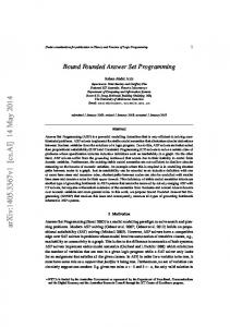
ΠX = {head (r) ← body + (r) | r ∈ Π, body − (r) ∩ X = ∅}. With these formalities at hand, we can define answer set semantics for logic programs: A set X of atoms is an answer set of a program Π if Cn(ΠX ) = X. This definition is due to [22], where the term stable model is used; the idea traces back to [45]. In fact, one may regard an answer set as a model of a program Π that is somehow “stable” under Π. In other words, an answer set is closed under the rules of Π, and it is “grounded in Π”, that is, each of its atoms has a derivation using “applicable” rules from Π. For illustration, consider the program Π = {p ← p, q ← not p} . Among the four candidate sets, we find a single answer set, {q}, as can be verified by means of the following table:
Background
We restrict the formal development of ASP to propositional (normal) logic programs consisting of rules of the form p0 ← p1 , . . . , pm , not pm+1 , . . . , not pn ,
where n ≥ m ≥ 0, and each pi (0 ≤ i ≤ n) is an atom. Given such a rule r, we let head (r) denote the head, p0 , of r and body(r) the body, {p1 , . . . , pm , not pm+1 , . . . , not pn }, of r. Also, let body + (r) = {p1 , . . . , pm } and body − (r) = {pm+1 , . . . , pn }. The intuitive reading of such a rule is that of a constraint on an answer set: If all atoms in body + (r) are included in the set and no atom in body − (r) is in it, then head (r) must be included in the answer set. Answer sets as such are defined via a reduction to negationas-failure-free programs: A logic program is called basic if body − (r) = ∅ for all its rules. A set of atoms X is closed under a basic program Π if for any r ∈ Π, head (r) ∈ X whenever body + (r) ⊆ X. The smallest set of atoms which is closed under a basic program Π is denoted by Cn(Π) and constitutes the answer set of Π. For the general case, we need the concept of a reduct of a program Π relative to a set X of atoms:
(1)
X ∅ {p} {q} {p, q}
ΠX p q p p q p
← ← ← ← ← ←
p
Cn(ΠX ) {q}
p p
∅ {q}
p
∅
Seite 1
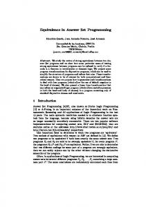
A noteworthy fact is that posing the query p or q to Π in a Prolog system leads to non-terminating situation due to its top-down approach. Analogously, we may check that the program Π1 = {p ← not q, q ← not p}
Let us first give a “generator”. To this end, we build upon the non-deterministic behavior observed on program Π1 . Also, we introduce an auxiliary atom q 0 (i, j) indicating that there is no queen at (i, j). Finally, we need a “domain predicate” d indicating the dimension of the chessboard. Accordingly, we obtain:
has the two answer sets {p} and {q}. X ∅ {p} {q} {p, q}
ΠX p q p q
← ← ← ←
d(X), d(Y ), not q 0 (X, Y )
(3)
0
←
d(X), d(Y ), not q(X, Y )
(4)
So, taking a 1×1 chessboard by adding d(1), we obtain from (3) and (4) two answer sets, {q(1, 1), d(1)} and {q 0 (1, 1), d(1)}, just as with program Π1 . Accordingly, we obtain by adding d(1) and d(2) a 2 × 2 chessboard, generating 16 answer sets, among which we find:
{p} {q} ∅
The two rules in Π1 are mutually exclusive and capture an indefinite situation: p can be added unless q has been added and vice versa. We show in the next section how this can be exploited in modeling problems in ASP. Unlike the previous examples, Π2 = {p ← not p}
{q 0 (1, 1), q 0 (1, 2), q 0 (2, 1), q 0 (2, 2), d(1), d(2)}
(2)
This can be done by introducing a new atom f and replacing (2) by rule f ← not f, p1 , . . . , pm , not pm+1 , . . . , not pn . Whenever the integrity constraint in (2) is violated by a candidate set this set is eliminated by the effect observed on program Π2 . The usefulness of integrity constraints can be observed by adding ← p to program Π1 . In fact, the integrity constraints ← p eliminates the original answer set {p} of Π1 , so that Π1 ∪ {← p} yields a single answer set {q}. Although general ASP is principally computationally complete, that is, it can simulate arbitrary Turing machines [6], one usually deals with decidable fragments. Commonly, we consider rules with variables that are taken as abbreviations for all ground instances over a finite set of constants. The propositional fragment of ASP defined above allows for encoding all decision and search problems within NP [48, 33].
q
{q(1, 1), q 0 (1, 2), q 0 (2, 1), q(2, 2), d(1), d(2)}
q
{q(1, 1), q(1, 2), q(2, 1), q(2, 2), d(1), d(2)}
q q
(6)
q q q
(7) (8)
Now, the “tester” must eliminate candidate sets in which queens are positioned on the same row, column, or diagonal. This can be done by means of the following integrity constraints: ←
q(X, Y ), q(X 0 , Y ), X 0 6= X, d(X), d(Y ), d(X 0 ), d(Y 0 )
(9)
←
q(X, Y ), q(X, Y 0 ), Y 0 6= Y, d(X), d(Y ), d(X 0 ), d(Y 0 )
(10)
←
q(X, Y ), q(X 0 , Y 0 ), |X − X 0 | = |Y − Y 0 |, (11) X 0 6= X, Y 0 6= Y, d(X), d(Y ), d(X 0 ), d(Y 0 )
In fact, all rules rule out candidate set (8). Rule (11) eliminates set (7). However, none of them accounts for the requirement that n queens must be put on the board. This can be achieved by the following pair of rules.
hasq(X)
Modeling
The basic approach to writing programs in ASP follows a “generate-and-test” strategy. First, one writes a group of rules whose answer sets would correspond to candidate solutions. Then, one adds a second group of rules, mainly consisting of integrity constraints, that eliminates candidates representing invalid solutions. As an example consider the well-known n-queens problem. The goal is to place n queens on an n × n chessboard so that no two queens appear on the same row, column, or diagonal. Let us represent the positioning of the queens by atoms of the form q(i, j), where 1 ≤ i, j ≤ n. That is, an atom q(i, j) represents that a queen is at position (i, j).
(5)
{q(1, 1), q 0 (1, 2), q 0 (2, 1), q 0 (2, 2), d(1), d(2)}
admits no answer set. Interestingly, Π2 offers a straightforward way to model integrity constraints of form
3
←
q (X, Y )
Cn(ΠX ) {p, q}
← p1 , . . . , pm , not pm+1 , . . . , not pn .
q(X, Y )
←
d(X), hasq(X)
←
d(X), d(Y ), q(X, Y )
The two latter rules eliminate candidate sets (5) and (6).
4
Language Extensions
Classical negation. Normal logic programs provide negative information implicitly through the closed world assumption [44]. Consider the following rule: cross ← not train. If train is not derivable, the atom cross becomes true. But this may lead to a disaster because you have no explicit information that there really is no train. An alternative would be to use an explicit negation operator ¬. Then we can express the previous rule as follows: cross ← ¬train.
Seite 2
An atom p or a negated atom ¬p is called a literal. Logic programs with literals are called extended logic programs [22]. An extended logic program is contradictory [5] if complementary literals, e.g. train and ¬train, are derivable. In that case, one obtains exactly one answer set, viz the set of all literals. If a program is not contradictory, the definition of answer sets of extended logic programs carries over from normal programs. Classical negation can be eliminated by a polynomial transformation, replacing each negated atom ¬p by a new atom p0 and adding the rules, q ← p, p0
and
q 0 ← p, p0 ,
(12)
for each atom p and q. The rules in (12) generate the set of all literals in case of contradictory programs. For preserving only consistent answer sets, we may add constraints ← p, p0 for each atom p, instead of the rules in (12). Disjunctive logic programs extend normal programs by disjunctive information in the head of a rule [22]. More precisely, the head of a rule is a disjunction q0 ; . . . ; qk for atoms qi , where 0 ≤ i ≤ k. E.g. p; q expresses that “p is true or q is true”. Letting head (r) = {q0 , . . . , qk }, a set of atoms X is closed under a basic program Π if for any r ∈ Π, head (r) ∩ X 6= ∅ whenever body + (r) ⊆ X. The definition of ΠX carries over from normal programs. An answer set X of a disjunctive logic program is a ⊆- minimal set of atoms being closed under ΠX . For example, the disjunctive logic program Π = {p; q ←} has the answer sets {p} and {q}. The set {p, q} is closed under Π{p,q} , but it is not an answer set of Π since it is not ⊆-minimal. Observe that adding the rules p ← and q ← to Π makes {p, q} the only answer set of Π ∪ {p ←, q ←}. If we use disjunction in the n-queens problem, rules (3) and (4) can be replaced by one rule: q(X, Y ); q 0 (X, Y )
←
d(X), d(Y )
The usage of disjunction raises the complexity of the underlying decision problems, e.g. deciding whether there exists an answer set X for a given atom p such that p ∈ X is ΣP 2 complete [18]. Nested logic programs are logic programs where the bodies and heads of rules may contain arbitrary boolean expressions formed from propositional atoms and the symbols > (true) and ⊥ (false) using negation-as-failure (not), conjunction (,), and disjunction (;) [30]. Answer sets are similarly defined as for disjunctive programs under regard that every boolean expression must be satisfied in the sense of classical logic and that the reduct ΠX is operating on boolean expressions. For illustration, consider nested program Π = {(p; not p) ←}. Taking X = ∅, we obtain Π∅ = {(p; >) ←} as reduct and ∅ as the only ⊆- minimal set being closed under Π∅ , that is, the boolean expression (p; >) is trivially satisfied by X = ∅. For X = {p}, we get Π{p} = {(p; ⊥) ←} and {p} as the ⊆-minimal set satisfying the expression (p; ⊥). Hence, ∅ and {p} are the answer sets of nested program {(p; not p) ←}. In the n-queens problem, rules (3) and (4) can be replaced by q(X, Y ); not q(X, Y ) ← d(X), d(Y ) , where the usage of nested expressions avoids using auxiliary predicate q 0 .
Nested programs can be polynomially translated into disjunctive programs [39]. Cardinality constraints are extended literals [49]. They are of the form l {q1 , . . . , qm } u, for m ≥ 1, where l, u are lower and upper bounds on the cardinality of subsets of {q1 , . . . , qm } satisfied in an encompassing answer set. They can appear in the head or in the body of a rule. A cardinality constraint is satisfied in an answer set X, if the number of atoms from {q1 , . . . , qm } belonging to X is between l and u. To ensure in the n-queens problem that exactly one queen is in every column j, we use the expression 1{q(1, j), . . . , q(n, j)}1, which can be abbreviated by 1{q(X, j) : d(X)}1, a so-called conditional literal [49]. Hence, the n-queens problem can be encoded with three rules, namely rule (11) and 1{q(X, Y ) : d(X)}1
←
d(Y )
(13)
1{q(X, Y ) : d(Y )}1
←
d(X),
(14)
where rules (13) and (14) ensure that there is exactly one queen in every column and row, respectively. Deciding whether a normal program with cardinality constraints has an answer set is NP-complete [49]. Preferences. The notion of preference is pervasive in commonsense reasoning, e.g. in decision making, in part because preferences constitute a very natural and effective way of resolving indeterminate situations. In the following, we will exemplarily consider preferences among rules and so-called ordered disjunctions. Rule preferences. A logic program with (static) preferences is a pair (Π,