A Gradient-Based Adaptive Learning Framework for Online Seizure ...

1

A Gradient-Based Adaptive Learning Framework for Online Seizure Prediction Shouyi Wang* Department of Industrial and Engineering, University of Texas at Arlington, Arlington, TX 76019, USA E-mail: [email protected] *Corresponding author

Manufacturing

Systems

Wanpracha Art Chaovalitwongse Department of Industrial and Systems Engineering, Department of Radiology at Medical Center, University of Washington, Seattle, WA 98195, USA E-mail: [email protected]

Stephen Wong Robert Wood Johnson Medical School, University of Medicine and Dentistry of New Jersey, New Brunswick, NJ 08901, USA E-mail: [email protected] Abstract: Most of the current epileptic seizure prediction algorithms require much prior knowledge of a patient’s pre-seizure electroencephalogram (EEG) patterns. They are impractical to be applied to a wide range of patients due to a very high inter-individual variability of EEG patterns. This paper proposes an adaptive prediction framework, which is capable of accumulating knowledge of pre-seizure EEG patterns by monitoring long-term EEG recordings. The experimental results on five patients indicate that the proposed prediction approach is effective to achieve a personalized seizure predication for each patient using a gradient-based adaptive learning framework. Keywords: adaptive seizure prediction; gradient-based learning; time series online monitoring. Reference to this paper should be made as follows: Wang, S., Chaovalitwongse W., and Wong, S. (2011) ‘A Gradient-Based Adaptive Learning Framework for Online Seizure Prediction’. Biographical notes: Shouyi Wang received a B.S. degree in Control Science and Engineering from Harbin Institute of Technology, Harbin, China, in 2003, and a M.S. degree in Systems and Control

2

S. Wang, W. Chaovalitwongse, and S. Wong Engineering from Delft University of Technology, Netherlands in 2005. Currently, he is a Ph.D. candidate at the Department of Industrial and Systems Engineering, Rutgers University. And he is also working as a research scientist at the Department of Industrial & Systems Engineering and the Integrated Brain Imaging Center (IBIC), University of Washington. His research interests include time series data mining, pattern discovery, machine learning, intelligent decisionmaking systems, multivariate time series modeling and forecasting. Wanpracha Art Chaovalitwongse received a B.S. degree in Telecommunication Engineering from King Mongkut Institute of Technology Ladkrabang, Thailand, in 1999 and M.S. and Ph.D. degrees in Industrial and Systems Engineering from University of Florida in 2000 and 2003, respectively. In 2004, he worked at the Corporate Strategic Research, ExxonMobil Research & Engineering, where he managed research in developing efficient mathematical models and novel statistical data analysis for upstream and downstream business operations. He was an Assistant Professor from 2005 to 2010 and an Associate Professor from 2010 to 2011 in the Department of Industrial & Systems Engineering, Rutgers University. Currently, he is an Associate Professor in the department of Industrial & Systems Engineering and the Department of Radiology at Medical Center, University of Washington. Stephen Wong received a B.S. degree in 1996 at the California Institute of Technology in Pasadena, CA. He obtained his M.D. at Duke University in the year 2000 in Durham, NC, and received subsequent medical training in neurology and epilepsy at the University of Pennsylvania Health System in Philadelphia, PA. He was the recipient of scholarship for a Master’s Degree in Translational Research, which he received in 2010, during which he studied signal processing and machine learning methods applied to clinical neurophysiology and electroencephalography. He is currently an assistant professor of neurology at UMDNJ-Robert Wood Johnson Medical School in New Brunswick, NJ, where he provides clinical care to patients with epilepsy, teaches medical students and residents, and performs computational research related to event detection in neurophysiology.

1 Introduction According to Engel and Pedley (1997), about 50 million people suffer from epilepsy, which is a chronic neurological disorder characterized by recurrent unprovoked seizures. Epileptic seizures generally occur without any warning, the shift between normal brain state and seizure onset is often described as an abrupt phenomenon. The seemingly unpredictability of epileptic seizures is one of the major causes of morbidity and stress in patients with epilepsy. Therefore, being able to identify pre-seizure symptoms could significantly improve the quality of life for these patients and can also open new diagnostic and therapeutic opportunities in epilepsy treatment. Over the recent years, there has been accumulating evidence indicating that a transitional pre-seizure state does exist prior to seizure onset. As stated in Delamont et al. (1999), pre-seizure symptoms such as irritability or headache

3 are frequently exhibited minutes, hours or even days prior to seizure onsets. Some other clinical findings also support the existence of a pre-seizure state, such as increases in cerebral blood flow, oxygen availability, and blood oxygen level-dependent signal, and changes in heart rate prior to seizure occurrence. The quantitative studies of the pre-seizure state are mostly based on EEG recordings from patients with epilepsy. For example, Lehnertz and Elger (1998) showed that the correlation dimension decreases prior to seizures. Quyen et al. (2003) reported a reduction in the dynamical similarity index before seizure occurrence. Iasemidis et al. (1997) noted premonitory pre-seizure changes based on the analysis of dynamical entrainment. Mormann et al. (2006) observed a pre-seizure drop in phase synchronization up to hours prior to seizure onset. In the past decades, many studies have been carried out aiming to predict epileptic seizures. Seizure predictability by EEG recordings has been confirmed by a number of groups (Elger and Lehnertz (1998); Lehnertz and Elger (1998); Quyen et al. (1999); Litt et al. (2001); Jerger et al. (2005)). An extensive survey of EEG-based seizure prediction techniques can be found in Mormann et al. (2007). Most of the current seizure prediction methods mainly have two steps. Firstly, EEG features are extracted from a sliding moving window. Then each window-EEG is classified as either pre-seizure or normal by comparing the extracted EEG features with the predefined threshold levels. Whenever a windowEEG is classified as pre-seizure, a warning alarm is triggered indicating that an impending seizure may occur within a pre-defined prediction horizon. These methods have shown good results for some patients. However, the reliability and repeatability of the results have been questioned when they were tested on other EEG datasets. Many of the earlier optimistic findings cannot be reproduced or achieved poor performance in extended EEG datasets in later studies as reported in Aschenbrenner-Scheibe et al. (2003). This is not surprising since the optimal threshold obtained from a few number of patients may not be appropriate to many others. Therefore, we regard the future perspective of a practical seizure prediction system with ‘optimized’ thresholds as unrealistic. Instead, we would conjecture the most promising approach should be an intelligent method that can be autonomously adaptive to each individual patient with learning ability. Inspired by the great reinforcement learning ability of human beings, we attempt to construct an adaptive learning system, which could interactively learn from a patient, and is capable of improving prediction performance over time. In addition, many of the current seizure prediction studies are basically to solve a classification problem for normal and pre-seizure EEG data. The resulting methods do not take sufficient account of the online monitoring property in their prediction methods. The proposed adaptive framework successfully combines the reinforcement learning concept, online monitoring and adaptive control theory to achieve the online patient-specific seizure prediction. This work is among the pioneering attempts to tackle the greatly challenging task of online seizure prediction. The prediction framework avoids a sophisticated threshold-tuning process, and largely enhances the adaptability of the current prediction techniques. The autonomous self-adaptation property of the system makes it convenient to use for end users, such as physicians and patients. The outcome of this study would shed some light on the perspective reliable online seizure prediction techniques. It

4

S. Wang, W. Chaovalitwongse, and S. Wong

may also improve the medical diagnosis and prognosis in other brain diseases, such as sleep disorders and cognitive disorders. This paper is organized as follows. Section 2 presents the experimental methods, including EEG collection, feature extraction, and the proposed adaptive learning framework. The experimental results are provided in Section 3, and we conclude the paper in Section 4.

2 Methods All the experiments were performed on an Intel Xeon 2.0 GHz 64-bits workstation with 16 gigabytes of memory running on Windows Server 2003. All calculations and algorithms were implemented and run on MATLAB R2009b. Both default Matlab programs and user-designed programs were used in the experiments.

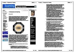
2.1 Data Collection Intracranial EEG recordings from five epileptic patients with temporal lobe epilepsy were analyzed in this study. The placement of the EEG electrodes is shown in Figure 1, which is a modified image of the inferior transverse view of the brain from Potter (2006). The recorded EEG data is summarized in Table 1. The EEG recordings consist of 26 standard channels, and the durations are ranged from 3 to 13 days. A total of 89 seizures over 43 days were recorded. The starting and the ending time points of seizure onsets were determined by experts.

Subduralelectrodestripsare placedover: leftorbitofrontal(LOF) rightorbitofrontal(ROF) leftsubtemporal(LST) rightsubtemporal(RST)cortex Depthelectrodesareplacedin: lefttemporaldepth(LTD) righttemporaldepth(RTD)

Figure 1

The interior transverse view of the brain and the placement of the 26 EEG electrodes.

2.2 Data Preprocessing & Feature Extraction Many feature extraction techniques have been developed to analyze EEG signals, such as time-domain analysis, frequency-domain analysis, time-frequency analysis, and spatial-temporal analysis. A comprehensive review of various EEG processing

5 Table 1

Summary of the Analyzed EEG Data

Patient Number Duration of of EEG Electrodes (days) 1 2 3 4 5 Total

26 26 26 26 26

3.55 8.85 13.13 6.09 11.53 43.15

Number of Seizures 7 22 17 23 20 89

Seizure Rate (per hour) 0.082 0.104 0.054 0.157 0.061

methods can be found in Stam (2005). Since EEG signals are highly nonstationary and seemingly chaotic, there has been an increasing interest in analyzing EEG signals in the context of chaos theory according to Rapp et al. (1989). Chaos theory provides effective quantitative methods to measure EEG dynamics and discover the underlying chaos in the data. Several chaotic measures are commonly used in recent EEG literature, such as correlation dimension in Silva et al. (1999), largest Lyapunov exponent in Iasemidis et al. (2003), Hurst exponent in Dangel et al. (1999) and entropy in Quiroga et al. (2000). Among such measures, Lyapunov exponent, the average rate of divergence of two neighboring trajectories in phase space, is often considered as the most basic indicator of deterministic chaos (Vastano and Kostelich (1986)). Lyapunov exponents supply a direct measure of the degree of sensitivity to initial conditions for a dynamical system. For a n-dimensional dynamical system, there are n different Lyapunov exponents, λi . They measure the exponential rate of divergence of the different trajectories in the phase space. If one of the exponents is positive, it indicates that the two corresponding orbits defined by that exponent diverge exponentially. The magnitude of the exponents indicates the degree of divergence. It has been shown that the chaotic behavior of a dynamical system is usually sufficient to be characterized by the largest Lyapunov exponent instead of all the exponents. The largest Lyapunov exponent has been shown to be reliable and reproducible in Vastano and Kostelich (1986). In our previous studies, an estimation algorithm called short-term largest Lyapunov exponent (ST Lmax ) was developed to quantify EEG dynamics in Iasemidis et al. (2000). Along this line of research, we also employ ST Lmax to characterize raw EEG data in this study. The calculation of ST Lmax can be briefly described as follows. The initial step is to embed each channel of EEG signal in a p-dimensional phase space, and construct p-dimensional vectors X(ti ) = (x(ti )), x(ti + τ ), . . . , x(ti + (p − 1)τ ), where ti is the time point, τ is the selected time lag between the components of each vector in the phase space, and p is the selected dimension of the embedding phase space. Define N the number of local ST Lmax s that will be estimated within a duration T data segment, then the

6

S. Wang, W. Chaovalitwongse, and S. Wong

largest Lyapunov exponent is defined as the average of local Lyapunov exponents Lij in the phase space as follows: ST Lmax =

1 ∑ · Lij , N

(1)

N

and the local Lyapunov exponents Lij is defined by: Lij =

X(ti + ∆t) − X(tj + ∆t) 1 · log2 , ∆t X(ti ) − X(tj )

(2)

where ∆t is the evolution time for the vector difference δXi,j (0) = |X(ti ) − X(tj )| to evolve to the new difference δXi,j (∆t) = |X(ti + ∆t) − X(tj + ∆t)|. More details of the estimation of ST Lmax can be found in Iasemidis (1991).

2.3 Adaptive Seizure Prediction Framework The proposed adaptive seizure prediction framework is illustrated in Figure 2. The continuous multichannel EEG data were analyzed by a sliding moving window. The window had a size of 10 min and moved with a 50% overlap each step. Two baselines of normal and pre-seizure states were constructed to classify the windowEEGs using a KNN method. All the baseline samples and window-EEGs were represented in terms of multichannel time profile of ST Lmax s. Based on prediction feedbacks (correct or incorrect), the two baselines were updated according to a reinforcement learning procedure. The adaptive seizure prediction system is discussed in detail in the following.

2.3.1 Baseline Construction & Initialization To start our prediction system, we need to initialize the pre-seizure and normal baseline samples. The selection of baseline samples highly depends on the presumed time length of pre-seizure period, which is often used as prediction horizon in seizure prediction literature. So far little is known to define pre-seizure duration, which has been reported between a few minutes and several hours prior to seizure onsets. The prediction horizon for epileptic seizures is still an open question in epilepsy research. In this study, we tried three prediction horizons, which are 30 min, 90min, and 150min, respectively. If we denote the prediction horizon at H minutes, then the EEG recordings can be divided into the following three periods: • Pre-seizure period: 0-H min preceding a seizure onset. • Post-seizure period: 0-20 min after a seizure onset. • Normal period: between pre- and post-seizure periods. The post-seizure period was set at 20 minutes based on the observations of the EEG recordings. The EEG signals generally recovered to normal patterns 20 minutes after the seizure onsets in all the five patients. In addition, the initial

7 Pre-seizure Period Hmin

Post-seizure Period

Normal Period

20min

Hmin

20min

MovingWindow

Seizure Onset

Seizure Onset Extractioinof

BaselineofNormalState

STL max

BaselineofPre-seizureState

MakePredictionBasedona KNN-basedDecision-MakingProcedure

PredictionEvaluationuntilOnePredictionHorizon LateroraSeizureOnset,whicheveroccursfirst.

Gradient-BasedWeight&BaselineUpdating

Figure 2

Schematic structure of the adaptive prediction system.

samples of the two baselines were randomly chosen from the normal and preseizure period preceding the first seizure onset. The length of the baseline samples is equal to that of the moving window. Since there is no guideline available to determine the number of samples in each baseline, we tentatively stored a fixed number of 50 samples in each baseline.

2.3.2 KNN Similarity Measure With baselines for normal and pre-seizure states, it is intuitive and practical for physicians to decide the class of a window-EEG based on its degree of similarity between the two baselines. For this purpose, KNN is the best choice because it classifies a new unlabeled sample by comparing it with all the samples of the two baselines. Thus, we employed KNN method to find the K best matching samples in each of the two baselines and compare them to make a decision. A KNN method has to use similarity measures to quantify the closeness between a moving-window EEG and baseline samples. We employed three frequently used similarity measures for time series data. If we denote two time series of ST Lmax as X and Y with equal length of n, then the three types of distances are briefly described as follows. ∑n • Euclidean distance (EU): EDxy = p=1 (xp − yp )2 /n.

8

S. Wang, W. Chaovalitwongse, and S. Wong ∑n √ • T-statistical distance (TS): T Sxy = p=1 |xp − yp |/ nτ|X−Y | , where τ|X−Y | is the sample standard deviation of the absolute difference between the time series X and Y . • Dynamic time warping (DTW): DTW measures similarity based on the best possible alignment or the minimum mapping distance between two time series. A detailed calculation of DTW can be found in Senin (2008).

Once a similarity measure is chosen, the distance between a window-EEG and a baseline sample, denoted as window-sample distance, can be obtained as follows:

dpre,i =

M ∑

j j distance(Spre,i , Smw ),

(3)

j j distance(Sint,i , Smw ),

(4)

j=1

dint,i =

M ∑ j=1

j j where M =26 is the number of EEG channels. Spre,i and Sint,i is the jth channel j of the ith pre-seizure and normal baseline sample, respectively; Smv,i is the jth channel of the window-EEG epoch. dpre,i and dint,i denote the distance between the window-EEG and the ith sample in the pre-seizure and normal baseline, respectively. The term distance in the above formula represents a time series distance measure, which can be EU, TS, or DTW in this paper.

2.3.3 KNN Prediction Procedure Four choices of K were employed, which were three, seven, half, and all of the baseline samples, respectively. For a specific value of K, the weighted summation of K nearest window-sample distances in a baseline was considered as the distance between the window-EEG and that baseline. We call the two distances as windownormal distance and window-preseizure distance, respectively. For each windowEEG, its distances to the two baselines can be calculated as follows: K Dpre =

K ∑

αk dpre,k ,

(5)

βk dint,k ,

(6)

k=1 K Dint =

K ∑ k=1

K K where Dpre and Dint are the window-preseizure distance and window-normal distance, respectively. dpre,k and dint,k are the window-sample distances of the kth sample of the K nearest neighbors in the pre-seizure and normal baseline, respectively. αk and βk are the weights of the kth sample in the pre-seizure and normal baseline, respectively; In the beginning, the initial weights of all baseline samples were equal, which are given by:

αi = βi =

1 , i = 1, . . . , n, n

(7)

9 n=50 is the number of samples in each baseline. We assume that different baseline samples may have different power in decision-making. The ‘importance’ of a baseline sample can be represented by a weight associated it. The weights of the baseline samples are updated through a gradient-based learning rule which will be discussed in a later part of this paper. Once the two baseline-window distances are obtained, the prediction decision can be made by: { K K 1, if Dpre /Dint ≤ h (trigger a warning), predictor = 0, otherwise (no warning), where the threshold h = 1 by default. The schematic structure of the KNN prediction rule is illustrated in Figure 3.

Pre-seizure Baseline

d pre,1 d pre,2 : d int,n

SelectK Nearest Neighbo rs If ,trigger D awar < Dning. K pre

Multichannel STL max

Normal Baseline

d int,1 d int,2 :

:

d pre,n

Figure 3

K int

Otherwise,nowarning. SelectK Nearest Neighbo rs

A demonstration of the KNN-based prediction rule.

2.3.4 Evaluation of a Prediction Result If the prediction horizon is H min, then the feedback of each prediction outcome can be classified into one of the following four categories: • True positive (TP): if predictor = 1 and a seizure occurs within H minutes after the prediction. • False positive (FP): if predictor = 1 and no seizure occurs within H minutes after the prediction. • True negative (TN): if predictor = 0 and no seizure occurs within H minutes after the prediction. • False negative (FN): if predictor = 0 and a seizure occurs within H minutes after the prediction. The concept of the prediction evaluation is also illustrated in Figure 4 for a better explanation. Based on this definition, we can evaluate a prediction result by identifying its corresponding category. Accordingly, the baselines will be updated based on the categorical prediction evaluations. In the following, the adaptive learning mechanism will be presented.

10

S. Wang, W. Chaovalitwongse, and S. Wong

PredictionOutcome pre-seizure

Actual Figure 4

pre-seizure normal

normal

TP FP

FN TN

The categorization of a prediction outcome. Each prediction outcome can be categorized into one of the four subsets.

2.3.5 Gradient-Based Weight Update Rule The flowchart of the baseline update framework from delayed prediction feedback is illustrated in Figure 5. Let r ∈ (0, 1) denote the learning rate to control the update size for the weights, then the gradient-based weight update rules are represented as follows: • For cases of TP & FN, the weight update rule is: αi = αi (1 −

dpre,i − dpre ) × r, dpre

(8)

βi = βi (1 +

dint,i − dint ) × r. dint

(9)

• For cases of FP & TN, the weight update rule is: αi = αi (1 +

dpre,i − dpre ) × r, dpre

(10)

βi = βi (1 −

dint,i − dint ) × r, dint

(11)

∑n ∑n where ∀i = 1, 2, . . . , n, dpre = i=1 dpre,i /n, and dint = i=1 dint,i /n. Since the above update rule cannot guarantee that the summation of the sample weights in one baseline equals to 1, we normalized the obtained new weight vectors after each update as follows: α = α/ β = β/

n ∑ i=1 n ∑

αi ,

(12)

βi .

(13)

i=1

2.4 Baseline Sample Update Rule After each weight update, the weights of ‘good’ samples are increased while the weights of ‘bad’ samples are decreased by the gradient-based weight update method. The weights indicate the ‘importance’ of the corresponding baseline

11 Look-backwardBaselineUpdate AnOldMovingWindow WaitingtobeEvaluated

CurrentMovingWindow PredictionEvaluation

OnePredictionHorizon(Hmin)orLess(when aseizureoccurswithinthepredictionhorizon)

CaseI:

NoseizureoccurswithinPredictionHorizon

If

TN

> £

If

CaseII:

FP AseizureoccurswithinPredictionHorizon TP

If