A graph decompositionbased approach for water distribution network ...

WATER RESOURCES RESEARCH, VOL. 49, 2093–2109, doi:10.1002/wrcr.20175, 2013

A graph decomposition-based approach for water distribution network optimization Feifei Zheng,1 Angus R. Simpson,1 Aaron C. Zecchin,1 and Jochen W. Deuerlein1,2 Received 31 May 2012; revised 27 February 2013; accepted 2 March 2013; published 24 April 2013.

[1] A novel optimization approach for water distribution network design is proposed in this paper. Using graph theory algorithms, a full water network is first decomposed into different subnetworks based on the connectivity of the network’s components. The original whole network is simplified to a directed augmented tree, in which the subnetworks are substituted by augmented nodes and directed links are created to connect them. Differential evolution (DE) is then employed to optimize each subnetwork based on the sequence specified by the assigned directed links in the augmented tree. Rather than optimizing the original network as a whole, the subnetworks are sequentially optimized by the DE algorithm. A solution choice table is established for each subnetwork (except for the subnetwork that includes a supply node) and the optimal solution of the original whole network is finally obtained by use of the solution choice tables. Furthermore, a preconditioning algorithm is applied to the subnetworks to produce an approximately optimal solution for the original whole network. This solution specifies promising regions for the final optimization algorithm to further optimize the subnetworks. Five water network case studies are used to demonstrate the effectiveness of the proposed optimization method. A standard DE algorithm (SDE) and a genetic algorithm (GA) are applied to each case study without network decomposition to enable a comparison with the proposed method. The results show that the proposed method consistently outperforms the SDE and GA (both with tuned parameters) in terms of both the solution quality and efficiency. Citation: Zheng, F., A. R. Simpson, A. C. Zecchin, and J. W. Deuerlein (2013), A graph decomposition-based approach for water distribution network optimization, Water Resour. Res., 49, 2093–2109, doi:10.1002/wrcr.20175.

1.

Introduction

[2] The optimization of water distribution network (WDN) design has been investigated over the past few decades, and a number of optimization techniques have been developed to tackle WDN optimization problem. These include linear programming (LP) [Alperovits and Shamir, 1977], nonlinear programming (NLP) [Fujiwara and Khang, 1990], and evolutionary algorithms (EAs) [Dandy et al., 1996; Montesinos et al., 1999; Reca and Martınez, 2006; Maier et al., 2003; Tolson et al., 2009; Suribabu, 2010; Zheng et al., 2013a]. However, it has been found that each optimization algorithm has its own advantages and disadvantages. [3] For LP and NLP, optimal solutions can be located efficiently, while only local minimums are provided. EAs are able to find good quality solutions but are computationally expensive. A number of advanced methods have been

1 School of Civil, Environmental and Mining Engineering, University of Adelaide, Adelaide, South Australia, Australia. 2 3S Consult GmbH, Karlsruhe, Germany.

Corresponding author: F. Zheng, School of Civil, Environmental and Mining Engineering, University of Adelaide, Adelaide, SA 5005, Australia. (feifei.zheng@ adelaide.edu.au) ©2013. American Geophysical Union. All Rights Reserved. 0043-1397/13/10.1002/wrcr.20175

proposed to reduce the computational intensity required by EAs in terms of WDN optimization [van Zyl et al., 2004; Tu et al., 2005; Keedwell and Khu, 2005; Reis et al., 2006]. Combining optimization techniques with water network decomposition is one of those advanced methods. [4] Normally, a WDN can be viewed as a connected graph G(V,E), where V is a set of links and E is a set of nodes in the WDN. Thus, it is natural to introduce graph theory algorithms to facilitate WDN analysis. Traditionally, graph theory was used for water network connectivity and reliability analysis. Gupta and Prasad [2000] used linear graph theory for the analysis of the pipe networks. Deuerlein [2008] proposed a graph theory algorithm to decompose a WDN into forests, bridges, and blocks. This method provides a tool to simplify complex WDNs and provides a better understanding of the interactions between their different parts of the network. [5] In terms of WDN optimization, Kessler et al. [1990] developed a graph theory based algorithm to optimize the design of WDNs. In their work, the design process consisted of three distinct stages. In the first stage, alternative paths were allocated using graph theory algorithms. In the second stage, the minimum hydraulic capacity (diameters) of each path was determined using an LP model. In the third stage, the obtained solution from the second stage was tested by a network solver for various demand patterns. [6] Sonak and Bhave [1993] introduced a combined graph decomposition-LP algorithm for WDN design. In

2093

ZHENG ET AL.: DECOMPOSITION METHOD FOR OPTIMIZING NETWORKS

this combined algorithm, all the trees of the looped WDN were first identified by a graph theory algorithm and optimized by a LP, allowing the global optimum tree solution to be located. The final optimal solution for the original WDN was then determined by assigning the chords of the global optimum tree the minimum allowable pipe diameters. Savic and Walters [1995] used graph theory to partition a water network into ‘‘tree’’ and ‘‘cotree’’ to enable an optimization problem that involved minimizing the heads by setting regulation valves. [7] Kadu et al. [2008] proposed a genetic algorithm (GA) combined with a graph theory algorithm to optimize water distribution systems. In their method, graph theory is used to identify the critical path for each node in order to reduce the search space for the GA. Krapivka and Ostfeld [2009] proposed a coupled GA-LP scheme for the least cost pipe sizing of water networks. A spanning tree identification algorithm was introduced in their work. Zheng et al. [2011] proposed a combined NLP-DE algorithm to optimize WDNs. In this algorithm, a graph theory algorithm was first used to identify the shortest-distance tree for the original whole WDN. Then, an NLP was implemented to optimize the tree network. The optimal solution obtained from the NLP optimization was finally utilized to seed a DE to optimize the original whole network. [8] Improvements in terms of efficiency and solution quality have consistently been reported by researchers when these optimization techniques are combined with graph theory algorithms and applied to WDN case studies. It was observed that, for the existing graph theory based optimization techniques, graph theory is normally used to identify the critical path or the spanning tree for the WDN in order to facilitate optimization. [9] For the proposed method here, a complete WDN is decomposed into subnetworks (rather than spanning trees) based on the connectivity of the network’s components. The resulting subnetwork may consist of a single block, bridges to this block, and/or trees connected to this block. For relatively simple networks (such as networks that have only one block and multiple trees attached to this block (case studies 2 and 3 in this paper)), the trees can be viewed as subnetworks. The subnetwork containing the water supply node (reservoir) is designated the root subnetwork. The definitions of block, bridge, and tree for the water network are given by Deuerlein [2008], who described a block in a WDN as a maximal biconnected subgraph; a bridge is a link joining two disconnected parts of a graph; and a tree is a connected subgraph without any circuits or loops. [10] After the subnetworks have been identified, each one is represented as an augmented node, and these augmented nodes are connected using directed links to form a directed augmented tree (AT), in which the directed links are used to specify the subnetwork optimization sequence. In order to improve the efficiency of the optimization process, a preconditioning approach is developed to approximately optimize the subnetworks in order to produce an approximate optimal solution for the original full network. The obtained approximate solution is able to specify promising regions within the entire search space. A final optimization method is then used to exploit these promising regions in order to generate further improved solutions for the original full network.

[11] The proposed optimization method presented in this paper is suited for the water networks where the graph decomposition can be applied and the WDN has no pumps and multiple reservoirs. The outcome of the proposed method is a significant improvement over the state of the art for designing common WDNs, and at the same time, is a starting point for future improvements to be applied to any WDN configuration. The details of the proposed methodology are given later.

2.

Formulation of WDN Optimization Problem

[12] Typically, a single-objective optimization of a WDN is the minimization of system costs (pipes, tanks, and other components) while satisfying head constraints at each node. In this paper, the proposed graph decomposition based optimization method is verified using WDN case studies with pipes only. Thus, the formulation of the WDS optimization problem can be given by Minimize

np X F¼a Dbi Li ;

(1)

i¼1

[13] Subject to: Hkmin Hk Hkmax GðHk ;DÞ

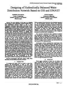
k ¼ 1; 2; :::; nj; ¼

Di 2 fAg;

0;

(2) (3) (4)

where F is the network cost that is to be minimized [Simpson et al., 1994]; Di is the diameter of the pipe i; Li is the length of the pipe i; a, b are specified coefficients for the cost function; np is the total number of pipes in the network; nj is the total number of nodes in the network; G(Hk, D) is the nodal mass balance and loop (path) energy balance equations for the whole network, which is solved by a hydraulic simulation package (EPANET2.0 in this study); Hk is the head at the node k ¼ 1,2 . . . .,nj; Hkmin and Hkmax are the lower and upper head limits at the nodes; and A is a set of commercially available pipe diameters.

3.

Methodology

[14] Four steps are involved in the proposed method for optimizing a WDN. [15] Step 1: The subnetworks for the full WDN that is being optimized are identified using a graph decomposition algorithm. [16] Step 2: A directed AT is built for the original full WDN. In the AT, the subnetworks appear as augmented nodes connected by directed links. The direction of the directed links in the AT determines the subnetwork optimization sequence in the proposed method. [17] Step 3: The subnetworks are then preconditioned using a DE algorithm to produce an approximate optimal solution for the original full network. [18] Step 4: The subnetworks are further optimized by a DE algorithm based on the approximate optimal solution obtained in Step 3. [19] The details of each step are as follows.

2094


Figure 1. An example of 27-pipe water network decomposition. (a) The original water network (G). (b) The proposed decomposition results (S). 3.1. Subnetwork Identification for the Full Water Network (Step 1) [20] Deuerlein [2008] proposed a graph theory algorithm to decompose a water network graph (G) into forest, blocks, and bridges according to its connectivity properties. In the method proposed here, however, the original network graph (G) is decomposed into a series of subnetworks (S). Each of the subnetworks may consist of one block, bridges to this block and trees attached to this block if applicable, or purely trees (if blocks are not applicable) [21] Figure 1 illustrates the decomposition results of a water network using the proposed new method. For the WDN (G) given in Figure 1a, six subnetworks are identified specified as follows by a set of nodes and pipes, including S1 ¼ {a, b, c, d, v, 1, 2, 3, 4, 5}, S2 ¼ {e, f, 6, 7, 8,}, S3 ¼ {g, h, i, j, 9, 10, 11, 12, 13}, S4 ¼ {k, l, m, n, 14, 15, 16, 17, 18}, S5 ¼ {o, p, q, 19, 20, 21, 22}, and S6 ¼ {r, s, t, u, 23, 24, 25, 26, 27}. S1 is denoted as a root subnetwork as it includes the supply source node v of the original water network. [22] As shown in Figure 1b, each subnetwork contains one and only one block, bridges to this block if applicable, and the trees attached to this block if applicable. The subnetworks overlap at some nodes as can be seen from Figure 1, i.e., S1 \ S2 ¼ c, S2 \ S3 ¼ f, S2 \ S4 ¼ e, S4 \ S5 ¼ m, and S4 \ S6 ¼ n. In this study, nodes c, f, e, m, and n are denoted as subnetwork cut nodes (C), i.e., C ¼ {c, f, e, m, n}. A depth first search (DFS) is employed to identify subnetwork cut nodes [Tarjan, 1972; Deuerlein, 2008] to enable network decomposition. 3.2. Directed AT Construction for the Original WDN (Step 2) [23] In order to assist in visualizing the proposed optimization method, the decomposed water network G is reconstructed as a directed AT by imagining each of the subnetworks as an augmented node and connecting the augmented nodes using directed links. The directed augmented tree AT of water network G given in Figure 1a is presented in Figure 2. As shown in Figure 2, reflecting graph theory terminology, S1 is the root augmented node in the AT since subnetwork S1 is the root subnetwork in Figure 1. S2 and S4

are located in the middle of the AT, while S3, S5, and S6 are located at the leaves of the AT. [24] The AT is now used to illustrate the two novel features of the proposed optimization method, which are (i) the optimization is carried out for each subnetwork separately (rather than for the original full network as a whole) in a predetermined sequence specified by the directed links in the AT and (ii) each subnetwork design optimization incorporates the solutions for all the subnetworks that are immediately attached to this subnetwork based on the direction of the directed links in the AT. [25] Referring the novel feature (i), as specified by the directed links in the AT given in Figure 2, S3, S5, and S6 are first separately optimized, followed by S4 ; then S2 and finally is S1. That is, subnetwork optimization takes place from the leaves to the root of the AT, which is opposite to the flow direction of the AT (that is from the root to the leaves as the supply source node is included in the rootaugmented node). [26] In order to facilitate the implementation of the novel feature (ii), for each subnetwork represented by an augmented node in the AT, all the other subnetworks that are immediately attached to this subnetwork based on the direction of the directed links are defined as its correlated subnetworks . Based on this definition, the correlated subnetworks for each subnetwork given in Figure 2 is ’ (S1) ¼ {S2}, ’ (S2) ¼ {S3, S4}, . . . ’ (S3) ¼ 1, ’(S4) ¼ {S5, S6}, ’(S5) ¼ 1, and ’(S6) ¼ 1. Based on the novel feature (ii) of the proposed method, each subnetwork design optimization needs to include the solutions for all the subnetworks in its ’. [27] By applying the two novel features to the water network given in Figure 1 (its AT is presented in Figure 2), S3, S5, and S6 should first be individually optimized and they do not consider other networks during optimization since their ’ ¼ 1. Then, S4 is optimized while incorporating the solutions for S5 and S6 since ’(S4) ¼ {S5, S6}. Subsequently, S2 is optimized and S3 and S4 are included during the optimization (’(S2) ¼ {S3, S4}). Finally, S1 is optimized and S2 is included (’(S1) ¼ {S2}). [28] As previously mentioned, two distinct optimization steps are utilized in the proposed method when dealing

Figure 2. The directed AT of the water network G given in Figure 1a.

2095

ZHENG ET AL.: DECOMPOSITION METHOD FOR OPTIMIZING NETWORKS Table 1. Nodal and Pipe Information of N1 Link 1 2 3 4 5 6 7 8 9 10 11 12 13 14 15 16 17 18 19 20 21 22 23 24 25 26 27

Length (m)

Node

Water Demand (L/s)

800 750 600 485 452 478 492 562 145 785 456 325 148 478 528 400 258 547 500 200 200 900 654 698 250 700 254

v a b c d e f g h i j k l m n o p q r s t u

Reservoir 25 27 32 15 48 20 124 14 32 13 17 22 42 89 26 23 11 19 17 16 32

with the optimization design for a WDN, which are preconditioning optimization for the subnetworks (Step 3) and the final optimization for the subnetworks (Step 4). The details of these two proposed optimization algorithms are discussed in the later section. [29] The water network given in Figure 1a (denoted as N1) is used to illustrate the proposed optimization approach. The elevation of all the demand nodes is 10 m, and the head provided by the supply source node (v) is 45 m. The minimum head requirement for each demand node is 35 m. The water demands for each node and the length for each pipe are given in Table 1. The Hazen-Williams coefficient for each new pipe is 130. A total of 14 diameters ranging from 150 to 1000 mm are used for the N1 design. The pipe diameters and the cost for each diameter are given by Kadu et al. [2008].

3.3. Preconditioning Optimization for the Subnetworks (Step 3) [30] Three typical subnetworks can be defined for the decomposed network in the proposed method, including the subnetworks at the leaves (L(AT)), subnetworks in the middle of the directed augmented tree (M(AT)), and the root subnetwork (Rt(AT)). For the subnetworks represented by augmented nodes in Figure 2, {S3, S5, S6}2L(AT), {S2, S4} 2M(AT), and S12Rt(AT). [31] Subnetworks at the leaves [S2L(AT)] differ from other subnetworks as their ’ ¼ 1. The root subnetwork [S2Rt(AT)] is characterized by its known available head, since it includes the supply source node of the original WDN. The available heads of the subnetworks in the middle of the directed augmented tree (S2M(AT)) are unknown and their 6¼1, which are different from S2L(AT) and

S2Rt(AT). In the proposed method, the optimization process for each type of subnetwork varies. 3.3.1. Optimization for the Subnetwork at the Leaves of the AT [32] The subnetworks at the leaves (S2L(AT)) are first optimized in the proposed method. Since no supply source node exists for each S2L(AT), each subnetwork cut node connecting the S2L(AT) and the S2M(AT) is assumed to be a supply source node for S2L(AT). Therefore, the subnetwork cut nodes f, m, and n represent the supply source nodes for S3, S5, and S6, respectively, as shown in Figure 1b. [33] Since the available head (H) at a subnetwork cut node is unknown, a series of sequential heads (H) between Hmin and Hmax are assigned for the subnetwork cut node, where Hmin is the maximum value of all minimum required nodal heads across the whole subnetwork that is being optimized and Hmax is the allowable head provided by the supply source node of the original network. The logic behind setting the head range [i.e., H2(Hmin, Hmax)] is that no feasible solution can be found if the available head at the subnetwork cut node is smaller than the maximum value of the minimum head constraints at all subnetwork nodes, and the maximum head of the subnetwork cut node cannot be greater than the head of the supply source node. A series of different H, H2(Hmin, Hmax), with a particular interval (say 1 m) are used for the subnetwork cut node in order to enable subnetwork optimization. [34] For each value of H assigned to a subnetwork cut node, a differential evolution (DE) algorithm combined with a hydraulic simulation model (EPANET2.0) is used to optimize the subnetwork design, while satisfying the head requirements for each node within the subnetwork. The minimum pressure head excess Hexcess (Hexcess 0) across the subnetwork is obtained for each optimal solution associated with a particular value of H at the subnetwork cut node. This indicates that the head at the subnetwork cut node can be further reduced by Hexcess while maintaining the feasibility of this optimal solution. The head H at the subnetwork cut node is then adjusted to H , where H ¼ H Hexcess, which is the minimum head requirement at the subnetwork cut node for the optimal solution associated with the minimum pressure head excess Hexcess. [35] Consequently, a solution choice table (ST) is constituted for the subnetwork that is being optimized by assigning a series of different values of H to its assumed supply source node, subnetwork cut node. In the ST, H , optimal solution costs and the subnetwork configurations (pipe diameters) of optimal solutions are included, and each unique H is associated with a unique optimal solution (including the cost and the subnetwork configuration). [36] The subnetwork S6 in N1 is used to illustrate the proposed optimization method for the S2L(AT). The Hmin and Hmax values for S6 are 35 and 45 m, respectively, where Hmin is the maximum head requirement for all nodes across S6 (35 m) and the Hmax is the allowable head provided by the actual supply source node (45 m). A series of H ranging from 35 to 45 m with an increment of 1 m, i.e.,H ¼ f36; 37; 38; . . . ; 45g is used for the subnetwork cut node n to optimize the design for S6. Note that no feasible solution can be found if H ¼ 35 m is assigned to node n as the minimum head requirement for S6 is 35 m. Thus, the value of H ¼ 35 m is not included in the series of

2096

ZHENG ET AL.: DECOMPOSITION METHOD FOR OPTIMIZING NETWORKS Table 2. Optimal Solutions for S6 of N1 H at Subnetwork Cut Node n (m)

Minimum Pressure Head Excess Hexcess (m)

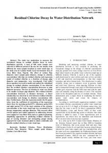
H¼ H Hexcess (m)

Cost of Optimal Solutions ($)

Pipe Diameters for Each Optimal Solutiona (mm)

0.014 0.231 0.157 0.120 0.397 0.513 0.790 0.402 1.402 0.160

35.986 36.769 37.843 38.880 39.603 40.487 41.210 42.598

155,487 130,288 115,622 108,175 105,079 98,175 95,079 92,032

450, 250, 300, 150, 300 400, 200, 300, 150, 250 350, 200, 250, 150, 300 350, 150, 250, 150, 250 350, 150, 250, 150, 200 300, 150, 250, 150, 250 300, 150, 250, 150, 200 300, 150, 200, 150, 200

44.840

89,168

250, 150, 200, 150, 250

36 37 38 39 40 41 42 43 44 45 a

The pipe diameters are for links 23–27 of N1 network (Figure 1a) from the first to the last pipe, respectively. Note that only one solution is recorded in the table for the identical solutions (having the same H , optimal cost, and pipe diameter for links).

H values assigned for the subnetwork cut node n. The optimal solution for each value of H, the minimum pressure head excess (Hexcess), and the H value for each optimal solution for S6 are given in Table 2. [38] As can be seen from Table 2, with values of H given at the subnetwork cut node n from the smallest to the largest (the first column of Table 2), values of H are also ordered from the smallest to the largest, while its corresponding optimal solution is ordered from the largest to the smallest in terms of cost. This is due to the fact that a lower cost solution is achieved if a higher head is provided at the subnetwork cut node. This solution choice table is denoted as STn since the subnetwork cut node n is the assumed supply source for S6. It is noted that the identical solutions (having the same H , optimal cost, and pipe diameters for links) are removed from the solutions choice table. For example, for heads of 43 and 44 m in STn, only one solution is left in the solution choice table. [39] Each S2L(AT) is optimized using the same approach as for S6 described above, and hence a solution choice table is constituted for each one after optimization. For N1 case study, in addition to S6, S3 and S5 are also subnetworks at the leaves of the directed augmented tree (see Figure 2). For S3 and S5, Hmin ¼ 35 m and Hmax ¼ 45 m, hence a series of values for H ¼ 36; 37; 38; . . . ; 45 are used for the subnetwork cut nodes f and m to optimize the design for the S3 and S5, respectively. As previously

explained, H ¼ 35 m is not assigned to the subnetwork cut nodes as no feasible solution can be found with this assumed head value (the minimum head requirement is 35 m for the N1 case study).The obtained solution choice tables for S3 and S5 are presented in Table 3 (the identical solutions have been removed from solution choice tables). 3.3.2. Optimization for the Subnetwork in the Middle of the AT [41] The optimization for the S2M(AT) is carried out once the optimization for S2L(AT) has been finished. For each S2M(AT), the water demands at each subnetwork cut node have to be increased by the flows in the directed links to this subnetwork that is being optimized (note the direction of the flows is opposite to the directed links). For the example given in Figure 1b, the water demands at subnetwork cut nodes f, m, and n [f2S2, {m, n}2S4, {S2, S4}2M(AT)] are increased by the flows in directed link l3, l4, and l5, respectively (see Figure 2), which are actually the demands of subnetworks S3, S5, and S6, respectively. The water demand at subnetwork cut node e is added by the flows in directed link l2, which are the total demands of subnetwork S4, S5, and S6, as shown in Figure 2. It is noted that each S2L(AT) is connected to the original entire network via only one subnetwork cut node, while each S2M(AT) is attached to the whole system with multiple subnetwork cut nodes.

Table 3. Solution Choice Tables for S3 and S5 of N1 Subnetwork Solution choice table for S3 [ST(f)] where node f is the assumed supply source node for S3

Solution choice table for S5 [ST (m)] where node m is the assumed supply source node for S5

H at Assumed Supply Source Node (m)

H ¼ H Hexcess (m)


Pipe Diameters for Each Optimal Solutiona (mm)

36 37 38 39 40 41 42 43 44, 45 36 37 38 39 40, 41, 42, 43, 44 45

35.845 36.939 37.765 38.886 39.916 40.903 41.547 42.575 43.054 35.995 36.864 37.925 38.649 39.710 44.607

90,200 73,900 67,620 63,553 62,915 60,483 57,995 57,357 55,778 74,686 64,603 62,469 57,717 55,583 51,623

500, 150, 350, 200, 200 400, 150, 300, 150, 200 400, 150, 250, 150, 200 350, 150, 250, 150, 150 300, 150, 250, 150, 200 400, 150, 200, 150, 150 350, 150, 200, 150, 200 300, 150, 200, 150, 200 300, 150, 200, 150, 150 350, 250, 150, 150 300, 200, 150, 150 300, 150, 150, 150 250, 200, 150, 150 250, 150, 150, 150 200, 200, 150, 150

a

The pipe diameters are for links 9–13 of N1 network (Figure 1a) in S3 and for links 19–22 of N1 network in S5 from the first to the last, respectively.

2097


[42] Among these subnetwork cut nodes attached to each S2M(AT), the one that is located at the upstream end based on the flow direction is assumed as a supply source. Thus, subnetwork cut nodes c and e are the assumed supply sources for S2 and S4, respectively, for the water network given in Figure 1. A series of different H, H2(Hmin, Hmax), with a particular interval (of again say 1 m) are assigned to the subnetwork cut node for optimizing the S2M(AT), which is the same approach as for optimizing S2L(AT) described in section 3.3.1. [43] It is important to note that for each S2M(AT), at least one subnetwork is located at its immediately adjacent downward side based on the direction of the directed links in the AT, i.e., 6¼1. In the proposed method, the optimization of each S2M(AT) needs to include all the subnetworks in its and the solutions for the subnetworks in its are selected from their corresponding solution choice tables during optimization. The formulation of the optimization problem for each S2M(AT) is given by Minimize

F 0 ¼ F ðS Þ þ

X

f ð’ðS ÞÞ;

S 2 MðATÞ;

(5)

[44] Subject to: min max HS;k HS;k HS;k

G HS;k ; Ds

0

k ¼ 1; ::::; nsj; ¼

(6)

0;

(7)

f ð’ðS ÞÞ 2 ST ð’ðS ÞÞ;

(8)

where F is the total cost (to be optimized); F ðS Þ is the cost of the subnetwork S (S2M(AT)) ; ’ðS Þ is all subnetworks in the ’ of S (the ’ is defined in section 3.2); X f ð’ðS ÞÞ is total costs for all other subnetworks in the ’; G(HS;k ,Ds ) is the nodal mass balance and loop (path) energy balance equations for the subnetwork S, which is handled by a hydraulic simulation package (EPANET2.0 in this study); HS;k is the nodal head of the node k ¼ 1, . . . , nsj; nsj is the number of nodes within the subnetwork S; min max and HS;k are the lower and upper head boundaries at HS;k the nodes of S; and ST ð’ðS ÞÞ is the solution choice tables of subnetworks in the ’. [45] As shown from equations (5)–(8), although the total costs of the S2M(AT) and all subnetworks in its ’ are to minimized, only the cost and nodal head constraints of the S2M(AT) are explicitly handled by an optimization algorithm (DE used in this study). This is because the optimal solutions for the subnetworks in the ’ [denoted as f ð’ðS ÞÞ] are selected from their corresponding solution choice tables ST ð’ðS ÞÞ during optimization (equation (8)). In addition, head constraints of subnetworks in the ’ are also handled by their corresponding solution choice tables. This is one of the novel aspects of the proposed optimization method. The details of the proposed method in terms of selecting optimal solutions from solutions choice tables and handling constraints during the optimization for the S2M(AT) are given as follows. [46] The optimization of S4 in N1 is used to illustrate the proposed methods for optimizing the S2M(AT). For the water network given in Figure 1 and its AT shown in Fig-

Figure 3. H versus the optimal solution cost for S6 of N1 (solution selection). ure 2, ’ðS4 Þ ¼ fS5 ; S6 g, and hence S5 and S6 are included when S4 is optimized. For S4 optimization, different values of H ¼ 36; 37; 38; . . . ; 45 are used for the assumed supply source e (Hmin ¼ 35 m and Hmax ¼ 45 m) and then a DE is employed to optimize the design for S4 for each H value. [47] The total cost, including the cost of S5, the cost of S6, and the cost of S4 is to be minimized for the DE applied to optimize S4 [’ðS4 Þ ¼ fS5 ; S6 g]. For each individual solution in the DE algorithm, the head at the subnetwork cut nodes m (Hm) and n (Hn) are tracked after the hydraulic simulation for S4 (EPANET2.0). Then the optimal solution for S5 and S6 are selected from their corresponding solution choice tables STm and STn based on assigning Hm and Hn to the subnetwork cut nodes m and n. As Hm and Hn may not precisely equal any particular H values in STm and STn, an approach is proposed in this study to select the appropriate optimal solutions based on the values of Hm and Hn. Figure 3 illustrates the details of this selection approach, and the values of H versus the optimal solution costs in the solution choice table STn for S6 is presented in Figure 3 to facilitate the explanation. [48] For each individual solution of the DE applied to optimize S4, Hn (head at the subnetwork cut node n) is obtained after hydraulic simulation for S4. Based on the value of Hn, three cases exist for selecting the optimal solution for S6, as shown in Figure 3: [49] Case 1: If Hn is smaller than the minimum H ½H ðAÞ in STn, the cost associated with the minimum H (the cost of solution A in Figure 3) is added to the total cost of this individual solution and the network configuration (pipe diameters) associated with ½H ðAÞ is assigned for S6. In addition, a penalty is applied to this individual solution as no feasible solution is found for S6. [50] Case 2: If Hn is greater than the maximum H ðH ðBÞÞ in STn, the cost associated with the maximum H (the cost of solution B in Figure 3) is added to the total cost of this solution and the network configuration (pipe diameters) associated with ½H ðBÞ is assigned for S6. [51] Case 3: If Hn is between two adjacent H values in STn, the solution has the H immediately smaller than the Hn is selected and its cost is added to the total cost of this individual solution. As shown in Figure 3, the solution C will be selected for S6 if the individual solution has a Hn between H ðC Þ and H ðDÞ, resulting in a pressure head excess of Hn H ðC Þ for S6. As such, the solution

2098

ZHENG ET AL.: DECOMPOSITION METHOD FOR OPTIMIZING NETWORKS Table 4. Solution Choice Table for S4 of N1

H at Subnetwork Cut Node e (m) 36 37 38 39 40 41 42 43 44 45

Pipe Diameters for Each Optimal Solutiona (mm) in the Solution Choice Table for S4 [ST(e)]

H ¼ H Hexcess (m)


S4

S5

S6

– 36.938 37.936 38.916 39.752 40.939 41.860 42.974 43.783 44.844

Infeasible 542,915 484,396 437,211 414,439 392,887 380,809 368,869 348,862 339,281

– 700, 600, 450, 600, 150 600, 500, 400, 600, 150 600, 500, 400, 500, 150 600, 450, 350, 450, 150 600, 450, 350, 450, 150 500, 450, 350, 500, 150 500, 500, 350, 400, 150 500, 400, 300, 400, 150 500, 400, 300, 400, 150

– 350, 250, 150, 150 350, 250, 150, 150 300, 200, 150, 150 300, 200, 150, 150 250, 200, 150, 150 300, 150, 150, 150 250, 200, 150, 150 250, 200, 150, 150 250, 150, 150, 150

– 450, 250, 300, 150, 300 450, 250, 300, 150, 300 400, 200, 300, 150, 250 400, 200, 300, 150, 250 350, 200, 250, 150, 300 350, 200, 250, 150, 300 350, 150, 250, 150, 250 350, 200, 250, 150, 300 350, 150, 250, 150, 250

a

The pipe diameters are for links 14–27 of N1 network from the first to the last, respectively (see Figure 1a).

selected from STn can be guaranteed to be feasible as the solution with H smaller than Hn is chosen. The network configuration (pipe diameters) associated with ½H ðC Þ is assigned for S6 in this case. [52] The approach described above is also used to include the cost of S5 when a DE is used to optimize S4. As such, although only the pipes in S4 are handled by the DE, the solutions in the DE actually include the total cost of S4, S5, and S6. Once the DE has converged to the final optimal solution for S4, the minimum pressure head excess Hexcess for this optimal solution is determined by Hexcess

¼ min½Hexcess ;

ðHm H ðSTm Þ;

ðHn H ðSTn Þ; (9)

where Hexcess is the minimum pressure head excess across all the demand nodes for S4 that is being optimized; H ðST m Þ and H ðST n Þ are the values of H associated with the solutions selected for S5 and S6 from ST m and ST n , respectively, based on the approach illustrated in Figure 3. The head H at the subnetwork cut node e is then adjusted to H , where H ¼ H Hexcess. [53] For each different value of H assigned to the subnetwork cut node e, the optimal cost solution for S4, S5, and S6 is obtained by the DE algorithm. In addition, the minimum pressure head excess Hexcess is obtained using equation (9), and hence the value of H (H ¼ H Hexcess) is obtained for each optimal solution. As such, a solution choice table for S4 is formed, in which, H , the optimal solution cost and subnetworks configuration (pipe diameters for S4, S5, and S6) of the optimal solution are included, which is presented in Table 4. [55] As shown in Table 4, a total of nine different feasible optimal solutions were found by the DE applied to S4 optimization with the heads at the assumed source node e being 36; 37; 38; . . . ; 45. No feasible solution was found with H ¼ 36 m assigned to node e. In the solution choice table ST(e) for S4, the values of H across the subnetworks of S4, S5, and S6, the total cost of S4, S5, and S6, the design for each of these three subnetworks are included. [56] As shown in Figure 2, ’ðS2 Þ ¼ fS3 ; S4 g, thus S3 and S4 are included when S2 is optimized in the proposed method. The subnetwork S4 is optimized before S2 as the optimization sequence in the proposed method is from the

leaves to the root based on the directed augmented tree. The approach described in Figure 3 was used to select the solutions for S3 and S4 from their corresponding solution choice tables when S2 is optimized. A similar method presented in equation (9) was utilized to obtain the Hexcess for each optimal solution of S2. [57] Since Hmin ¼ 35m and Hmax ¼ 45 m for S2, H ¼ 36; 37; 38; . . . ; 45 were used for the assumed supply source node c to optimize S2. In a similar way to that for S4, a solution choice table is formed for S2 after optimization, which is denoted as ST(c) as the subnetwork cut node c is the assumed supply source node. The final solutions in the ST(c) are the optimal solutions for S2, S3, and S4, which is actually the total optimal solutions for S2, S3, S4, S5, and S6 as the solutions in S4 have already included S5 and S6. The designs for the optimal solutions of S2, S3, S4, S5, and S6 are also included in the ST(c). [58] The formulation of the optimization problem given from equations (5)–(8) and the approach used for S4 optimization (Figure 3 and equation (9)) are employed to optimize each S2M(AT), thereby a solution choice table is constituted for each subnetwork in the middle of the directed augmented tree AT. 3.3.3. Optimization for the Subnetwork at the Root of the AT [59] The root subnetwork is the final one to be optimized in the proposed method. As the supply source node in the original full WDN is included in S2Rt(AT), the available head is known when optimizing S2Rt(AT). For the S2Rt(AT), ’ 6¼1 and hence the approach used for the optimization of S2M(AT) is also employed to deal with the optimization of the subnetwork at the root of the AT. For the example given in Figure 1, S12Rt(AT) and ’ðS1 Þ ¼ S2 , thus ST(c) is used to provide the optimal solution for S2 when S1 is optimized. [60] An approximate optimal solution with a cost of $1.021 million is obtained after S1 optimization, which is also the optimal solution for the whole N1 network. This is because S5 and S6 were included when S4 was optimized, S3 and S4 were included when S2 was optimized, and S2 was in turn included when S1 was optimized in the proposed method. Thus, the final optimal solutions from the optimization of S1 are the optimization results for the original full network N1.

2099


Figure 4.

H

versus the optimal solution cost for S6 of N1.

[61] During the preconditioning optimization for the subnetworks in the proposed method, a series of H with a relatively larger interval (H2(Hmin, Hmax)) is used for the subnetwork cut nodes (1 m in this study). This aims to approximately explore the search space of the original full network, thereby producing an approximate optimal solution. This approximate optimal solution is used to specify promising regions for the entire search space, allowing the next step (Step 4) of the final optimization for the subnetworks to be conducted. The final optimization for the subnetworks method is described in the next section. 3.4. Final Optimization of the Subnetworks (Step 4) [62] Based on the approximate optimal solution obtained by the preconditioning subnetwork optimization, an optimal head (H ) for each subnetwork cut node can be determined. An optimal head range