Nov 19, 2017 - obtain independent time series in graph frequency domain. We make .... Fourier Transform (GFT) [12] is defined as projecting a graph signal to ...
A GRAPH SIGNAL PROCESSING APPROACH FOR REAL-TIME TRAFFIC PREDICTION IN TRANSPORTATION NETWORKS Arman Hasanzadeh?
arXiv:1711.06954v1 [eess.SP] 19 Nov 2017
?
Xi Liu?
Nick Duffield ?
Krishna R. Narayanan ?
Byron Chigoy†
Texas A&M University, Dept. of Electrical & Computer Engineering, College Station, TX 77843, USA † Texas A&M Transportation Institute, College Station, TX 77843, USA ABSTRACT
Accurate real-time traffic prediction has a key role in traffic management strategies and intelligent transportation systems. Building a prediction model for transportation networks is challenging because spatio-temporal dependencies of traffic data in different roads are complex and the graph constructed from road networks is very large. Thus it is computationally expensive to build and run a prediction algorithm for the whole network. In this paper, we propose a method to address these challenges. First, we introduce a novel spatiotemporal clustering algorithm in order to split the large graph into multiple connected disjoint subgraphs. Then within each subgraph, we propose to use a Graph Signal Processing (GSP) approach to decouple spatial dependencies and obtain independent time series in graph frequency domain. We make predictions along independent graph frequencies using adaptive ARMA models and later transform the predicted time series along each graph frequency to the subgraph vertex domain. Evaluation of our model on an extensive dataset of fine-grained highway travel times in the Dallas– Fort Worth area shows substantial improvement achieved by our proposed method compared to existing methods. Index Terms— Graph Signal Processing, Graph Clustering, Big Data, Transportation Network 1. INTRODUCTION Intelligent Transport Systems (ITS) play an important role in managing traffic flows in transportation networks, especially with growing interest in using autonomous cars and routing applications. Accurate real-time traffic forecasting, especially after a crash or congestion events, can help ITSs to choose optimal routing and traffic managing strategy. Various datadriven approaches are used to forecast traffic in real-time. Existing frameworks for traffic prediction can be summerized under three categories – 1) regression based methods like Auto-Regressive Integrated Moving Average (ARIMA) [1], subset ARIMA [2] and multivariate ARMA [3], 2) supervised learning based methods such as Support Vector Regression (SVR) [4], Gaussian Process (GP) [5], Latent Space Modeling [6] and Deep Learning [7], 3) unsupervised learning based
methods like Principal Component Analysis (PCA) [8] and Robust PCA (RPCA) [7]. These works do not optimally use prior information regarding the spatio-temporal relationships in the data, and hence do not perform very well after occurrence of congestion or, are computationally very expensive (to learn the model or implement it) which make them inappropriate for real-time traffic prediction of very large networks. Graph Signal Processing (GSP) is an emerging technique for analyzing data points that are related by arbitrary graphs and GSP based techniques have recently been used to analyze traffic data [9], [10]. In our work, to deploy GSP framework, we model traffic flow as signals on vertices of a graph. We also use a recent result of Loukas et al. [11] in GSP area which introduced the notion of stationary time-vertex signal processing and showed that Minimum Mean-Square Error (MMSE) estimation problems on graphs can be solved with low complexity. Our approach and contributions in this paper can be summarized as follows: • We propose an efficient spatio-temporal clustering algorithm that splits the large graph into multiple connected disjoint subgraphs based on recurrent congestion spreading patterns in historical data. This helps to improve prediction accuracy and reduce computation complexity. • We propose to design adaptive prediction models for data defined on each subgraph separately. Prediction for each subgraph is done using adaptive ARMA models in graph frequency domain where time series defined at each graph frequency are independent of each other similar to the approach in [11]. • We evaluate our model using a large-scale traffic dataset collected from highways of Dallas–Forth Worth area which shows that our proposed model is more efficient and accurate than existing methods. 2. PROBLEM FORMULATION Each road in the network is represented by a node in a directed graph G = (V, E, Γ) where V is set of vertices, E is set of edges and Γ : E → R+ is the weight function. A directed edge (i, j) ∈ E exists if and only if road i is connected to road
Fig. 1. A schematic showing that the joint graph is the Cartesian product of the network graph and the time series graph. j by some intersection and vehicles can be transported from road i to road j. Equivalently, the graph G can be defined by a weight matrix, W . The (i, j) element of weight matrix is either zero if there is no edge from vertex i to vertex j or it equals to Γ(e) if e ∈ E and e connects vertex i to vertex j. The travel time (or speed) on a road can be considered as a time-varying signal associated with that road. Let x[t] : V → R|V| denotes the signal vector of the whole graph, where the i-th element represents the signal on road i. Then x[t] at each time is a time snapshot of the time-varying graph signal. A nice representation of discrete-time graph signals is to define them on a joint graph, which is the Cartesian product of the network graph and the time series graph1 of size T (where T is the number of time samples). Also, a signal defined on joint graph is represented by the matrix X ∈ R|V|×T , where the i-th row is associated with road i and the t-th column is x[t] for 1 ≤ t ≤ T . Therefore, the traffic prediction problem is defined as follows. Problem 1. Given graph G with weight matrix W and mtime-step historical observation on traffic X ∈ R|V|×m (i.e. (x[t−m], x[t−m+1], ..., x[t−1])), predict traffic for the next k time steps X ∈ R|V|×k (i.e. (x[t], x[t+1], ..., x[t+k −1])). 3. GRAPH SIGNAL PROCESSING 3.1. Graph Fourier Transform The classical Discrete Fourier Transform (DFT) can be considered as projection of a discrete-time signal (time series) on to the space whose bases are eigenfunctions of discrete Laplacian operator which is the same as Laplacian matrix of time series graph [12]. The Laplacian matrix of the time series graph is a circulant matrix whose eigenvectors are the same as columns of DFT matrix [13]. By extending this notion to arbitrary graphs, the Graph Fourier Transform (GFT) [12] is defined as projecting a graph signal to a space whose bases are the eigenvectors of Laplacian matrix of the graph. Let LG denotes the combinatorial Laplacian [14] of a directed graph G, defined as LG = 1 T 2 (Dout +Din −W −W ) where Dout and Din are out degree 1 Time
series graph here means the graph used to represent a time series as a graph signal. It is a directed path graph where each node shows a time step. The graph in the middle of Figure 1 is a time series graph.
Fig. 2. Schematic of ARM A(m, m) models for k-step preb = [GF T (Xt−m )|...|GF T (Xt )], diction of JWSS process. X eb e represent predicted signal in graph frequency doX and X main and predicted signal in vertex domain, respectively. N is the number of vertices. and in degree matrices, respectively. Also assume that UG and ΛG are eigenvector and diagonal eigenvalue matrices of LG , T respectively. More specifically, suppose LG = UG ΛG UG then the GFT and the Inverse GFT (IGFT) of a graph signal are defined as follows T GF T (x) = x ˆ = UG x,
IGF T (ˆ x) = x = U G x ˆ. Note that LG is a symmetric matrix thus complete eigendecomposition is always possible. This means that the number of graph frequencies (i.e. number of eigenvectors) is equal to the number of vertices of the graph, |V|. 3.2. Stationary Time-Vertex Signal Processing It is very well known that a time series is Time Wide-Sense Stationary (TWSS) if its expected value is constant and its second moment is only a function of the time difference. It is also straightforward to see that the covariance matrix of a TWSS process is a circulant matrix which is jointly diagonalizable with the Laplacian matrix of the time series graph (their eigenvectors are the same.). By generalizing the notion of TWSS to arbitrary graphs, Vertex Wide-Sense Stationarity (VWSS) [15] is defined as follows. Definition 1. A process defined on a graph is VWSS iff • E[x] = µx 1|V| = µx , • Σx = E[(x − µx )(x − µx )T ] is jointly diagonalizable with Laplacian matrix of the graph. Knowing the definition of TWSS and VWSS, Joint TimeVertex Wide-Sense Stationarity (JWSS) is defined as follows. Definition 2. A joint time-vertex process is JWSS iff at each time step, the graph signal is VWSS (i.e. X(:, t) = Xt is VWSS with respect to G for 1 ≤ t ≤ T ) and each of the time series defined on vertices of G are TWSS (i.e. X(i, :) is TWSS for all i ∈ {1, ..., |V|}). 3.3. Predicting Time-Varying Graph Signals It is well known that any TWSS process can be generated by filtering white noise. Based on this fact, one of most efficient
tools developed to predict a TWSS process is Auto Regressive Moving Average (ARMA) filters. ARMA filters try to predict the process by filtering samples of process and white noise in previous time steps. More formally, let y be a stationary time series. Then ARM A(m, q) model for predicting y at time t is defined as yet = c +
m X i=1
ai yt−i +
q X
bj εt−j
j=0
where yet is the predicted value of y at time t, εt is zero mean white noise at time t and c is a constant. While ARMA models are efficient for individual TWSS processes, predicting dependent time series together using ARMA can be computationally complex. More precisely, y and � will be vectors which makes the learning process complex and computationally expensive. Loukas et al. [11] proposed a model for predicting JWSS process which forecast signal in the graph frequency domain using independent ARMA models along each frequency. Independence in frequency domain is a result of joint time-vertex stationarity (a similar property is well known for TWSS processes). Figure 2 explains this model more precisely. It is important to note that using this method we are using data of all vertices to predict the signal at each vertex. In other words, spatio-temporal relation of adjacent vertices are hidden in every graph frequency components. While spatial relations can be captured by implementing multivariate ARMA, but it is computationally very expensive especially for large graphs. Here we only need N univariate ARMA models where N is number of vertices. The complexity of this model is linear in number of nodes and time steps [11]. There are two problems in directly using the approach in [11] for traffic prediction. First, in a typical traffic dataset with a very large graph, the signal defined on the graph is often non-stationary. Secondly, the computational complexity for a large graph is formidable. A common approach in the GSP literature to deal with the non-stationarity is to build local models for l-hop neighborhood of each vertex, for some value of l, instead of working with whole network. While this seems to be a promising way, it increases the computational complexity even more (even for small values of l for e.g., l = 5). Therefore, we propose to split the whole graph into multiple connected disjoint subgraphs by spatio-temporal clustering and then fitting prediction model on each individual subgraph.
important factor in clustering. More precisely, if congestion in one road spreads to an adjacent road, the two roads are considered to belong to the same cluster. First, we clarify the exact mathematical definition of congestion based on Travel Time Index (TTI). TTI is widely used in the transportation area to measure how congested a road is. TTI of a road is claculated as follows. Travel Time Index =
Current Travel Time of the Road . Free Flow Travel Time of the Road
Usually when TTI exceeds 1.7, it is a strong sign that the road is congested. Therefore we apply this threshold as the measure whether a road is congested or not. Definition 3. We say that the road i and road j are in the same spatio-temporal congestion pattern iff for some time t, firstly, (i, j) or (j, i) ∈ E and secondly congestion on road j is observed at time t and congestion on road i is observed at time t or t − 1 or vice versa. This definition makes sense since it is repeatedly observed that congestion on one road easily causes or serves as a result of congestion of its connected road with some time difference. This phenomenon occurs because the connected roads share traffic flows and thus easily get congested together. To obtain spatio-temporal congestion spreading patterns that satisfy the definition above, we propose the following fast iterative algorithm2 . At each time step, first we create the “congested graph” by removing the nodes with T T I < 1.7 and all the edges connected to these nodes from the whole network graph. Then we go through time and see if spreading patterns happened in consequtive times can be “merged” into one spreading pattern using the definition below. Definition 4. We say that spreading pattern 1 (SP1 ) that happened at time t can be merged with spreading pattern 2 (SP2 ) that happened at time t−1 if there is a common node between SP1 one-hop neighborhood of SP2 or vice versa. Once the congestion spreading patterns are known, we use a hierarchical graph clustering algorithm to find subgraphs. Suppose each congestion spreading pattern is represented as a data point in |V| dimension space as a binary vector of size |V| in which the i-th element shows whether the road i is in the that pattern or not. The distance between 2 patterns is defined as minimum length of shortest paths between any road in the first pattern and any road in the second pattern. Then at each iteration two patterns are combined (i.e. taking union of the roads in two patters as one cluster), if distance of two patterns are zero or one and the spatio-temporal data defined on the cluster subgraph after combination is JWSS. 4.2. Proposed Adaptive Predictor
4. PROPOSED PREDICTION MODEL 4.1. Proposed Spatio-Temporal Clustering “Spatio-temporal clustering” here means the algorithm considers the spatio-temporal congestion spreading patterns as an
Once the clusters are obtained, we propose using adaptive ARMA models along each graph frequency of clusters to 2 In fact, the algorithm quickly finds weakly connected components of the strong joint graph when spatio-temporal nodes with T T I < 1.7 and all of connected edges to them are removed.
5. NUMERICAL RESULTS AND DISCUSSION The traffic data used in this study originated from the DallasForth Worth area, with a graph comprising 4764 road segments in the highway network. The data represented timeseries of average travel times on each segment at a two-minute granularity over January–March 2013. We captured the spreading clusters for January and February 2013 from the dataset using our proposed algorithm. Log difference transformation was used to make the time series along each vertex TWSS. Also, the test proposed in [16] is deployed to check vertex stationarity. The signal is not stationary on whole graph but the signals defined on the subgraphs are almost JWSS since statistical behavior of roads on the same spreading cluster are similar. Adaptive ARM A(5, 5) models were trained using the same data. The Order of the ARMA models was obtained by testing a range of orders and the one chosen (m = q = 5) resulted in the best fitting. Adaptive ARMA models update if the normalized absolute error exceeds 10%. 10-step (20 minutes) real-time traffic prediction is performed on 100 randomly selected roads in the first week of March. To establish accuracy benchmarks, we consider two other common prediction models. First scheme is to build independent ARMA models for time series associated with each road. This naive scheme, ignores the spatial correlation of adjacent roads. Second benchmark scheme is Principal Component Analysis (PCA). In PCA, data vectors are projected to a lower dimensional data-driven subspace. Independent ARMA models are used to predict time series along each PCA component. We refer to the first model as temporal prediction and the second one as PCA prediction. In both of the models, ARM A(5, 5) has been deployed. Number of principal components is chosen such that 90% of the variance is covered. Mean Normalized Absolute Error (MNAE) is used as the measure for prediction accuracy. MNAE is defined as N T ˜ j) − X(i, j) 1 X X X(i, | |. N T i=1 j=1 X(i, j)
We noted that MNAE is 6.5% for temporal prediction, 4.3% for PCA prediction and 1.2% for our proposed method. Our proposed method reduced average error by a factor of four. It is important to note that because the number of nodes
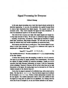
Temporal prediction PCA prediction Proposed spatio-temporal prediction
0.3 0.25 Normalized Absolute Error
forecast traffic. Adaptive ARMA have a significant advantage over ARMA in traffic prediction. Once a congestion or crash happens the statistics of process changes rapidly. The ARMA model results in high prediction error for a long time after congestion while adaptive ARMA can converge to a good predictor after a few time steps. Since we do real time prediction, it is easy to find real-time error. Once error exceeds a threshold (for e.g., 10%), we adapt the ARMA models to enhance fitting of the model.
0.2 0.15 0.1
5 · 10−2 0
0
200
400
600
800
1,000
Time Step Fig. 3. Normalized absolute error for 10-step prediction of the traffic of a road in 36 hours time span using different methods.
and time steps are very large, even half a percent is a good gain let alone improving by a factor of four. To have a better understanding of the predictors behavior, one road, which is in a cluster with 20 roads, is chosen. Normalized absolute error for 10-step prediction of the time series associated with this road in 36 hours time span is shown in Figure 3. When a congestion happens,a sharp increase appears in prediction error. While this sharp increase cannot be avoided, high prediction errors after a congestion will affect overall performance. As shown in Figure 3, temporal and PCA predictors cannot track the signal well after congestion (or it takes a long time for the error to decrease), while our proposed method the error decrease quickly after congestion. Our proposed method also improves prediction accuracy when there is no congestion by exploiting spatial correlation between neighboring roads.
6. CONCLUSION In this work, we introduced a new method for predicting traffic in road networks. In our proposed scheme, first a spatio-temporal clustering algorithm is deployed to determine congestion spreading clusters on graph. Then, an adaptive ARMA model for JWSS processes is used on each cluster independently to forecast the traffic. Numerical results showed that our proposed spatio-temporal prediction model improve the performance of temporal prediction and PCA prediction significantly. Another advantage of this method is that its low computational complexity, which is linear in the number of nodes and time steps.
7. REFERENCES [1] B. Pan, U. Demiryurek, and C. Shahabi. Utilizing realworld transportation data for accurate traffic prediction. In Data Mining (ICDM), 2012 IEEE 12th International Conference on, pages 595–604. IEEE, 2012. [2] S. Lee and D. Fambro. Application of subset autoregressive integrated moving average model for short-term freeway traffic volume forecasting. Transportation Research Record: Journal of the Transportation Research Board, (1678):179–188, 1999. [3] D. Pavlyuk. Short-term traffic forecasting using multivariate autoregressive models. Procedia Engineering, 178:57 – 66, 2017. [4] G. Ristanoski, W. Liu, and J. Bailey. Time series forecasting using distribution enhanced linear regression. In Pacific-Asia Conference on Knowledge Discovery and Data Mining, pages 484–495. Springer, 2013. [5] J. Zhou and A. KH. Tung. Smiler: A semi-lazy time series prediction system for sensors. In Proceedings of the 2015 ACM SIGMOD International Conference on Management of Data, pages 1871–1886. ACM, 2015. [6] D. Deng, C. Shahabi, U. Demiryurek, L. Zhu, R. Yu, and Y. Liu. Latent space model for road networks to predict time-varying traffic. arXiv preprint arXiv:1602.04301, 2016. [7] Y. Lv, Y. Duan, W. Kang, Z. Li, and F. Y. Wang. Traffic flow prediction with big data: A deep learning approach. IEEE Transactions on Intelligent Transportation Systems, 16(2):865–873, 2015. [8] W. Liu, Y. Zheng, S. Chawla, J. Yuan, and X. Xing. Discovering spatio-temporal causal interactions in traffic data streams. In Proceedings of the 17th ACM SIGKDD international conference on Knowledge discovery and data mining, pages 1010–1018. ACM, 2011. [9] D. M. Mohan, M. T. Asif, N. Mitrovic, J. Dauwels, and P. Jaillet. Wavelets on graphs with application to transportation networks. In 17th International IEEE Conference on Intelligent Transportation Systems (ITSC), pages 1707–1712, Oct 2014. [10] J. A. Deri and J. M. F. Moura. New York city taxi analysis with graph signal processing. In 2016 IEEE Global Conference on Signal and Information Processing (GlobalSIP), pages 1275–1279, Dec 2016. [11] A. Loukas and N.¨el Perraudin. Stationary time-vertex signal processing. arXiv preprint arXiv:1611.00255, 2016.
[12] D. I. Shuman, S. K. Narang, P. Frossard, A. Ortega, and P. Vandergheynst. The emerging field of signal processing on graphs: extending high-dimensional data analysis to networks and other irregular domains. IEEE Signal Processing Magazine, 30(3):83–98, 2013. [13] A. Sandryhaila and J. M. F. Moura. Big data analysis with signal processing on graphs: Representation and processing of massive data sets with irregular structure. IEEE Signal Processing Magazine, 31(5):80–90, Sept 2014. [14] F. Chung. Laplacians and the Cheeger inequality for directed graphs. Annals of Combinatorics, 9(1):1–19, 2005. [15] N. Perraudin and P. Vandergheynst. Stationary signal processing on graphs. IEEE Transactions on Signal Processing, 65(13):3462–3477, July 2017. [16] A. G. Marques, S. Segarra, G. Leus, and A. Ribeiro. Stationary graph processes and spectral estimation. CoRR, abs/1603.04667, 2016.