Yan Sun, Kongfa Hu, Zhipeng Lu, Li Zhao, Ling Chen. Department of Computer ... Yan Sun et al. / Physics Procedia 24 ... In [4] , Han introduced a method by ...
Available online at www.sciencedirect.com Available online at www.sciencedirect.com
Physics Procedia
Physics Physics ProcediaProcedia 00 (2011) 000–000 24 (2012) 1707 – 1714 www.elsevier.com/locate/procedia
2012 International Conference on Applied Physics and Industrial Engineering
A Graph Summarization Algorithm Based on RFID Logistics Yan Sun, Kongfa Hu, Zhipeng Lu, Li Zhao, Ling Chen Department of Computer Science and Engineering Yangzhou University Yangzhou 225009, China
Abstract Radio Frequency Identification (RFID) applications are set to play an essential role in object tracking and supply chain management systems. The volume of data generated by a typical RFID application will be enormous as each item will generate a complete history of all the individual locations that it occupied at every point in time. The movement trails of such RFID data form gigantic commodity flowgraph representing the locations and durations of the path stages traversed by each item. In this paper, we use graph to construct a warehouse of RFID commodity flows, and introduce a database-style operation to summarize graphs, which produces a summary graph by grouping nodes based on user-selected node attributes, further allows users to control the hierarchy of summaries. It can cut down the size of graphs, and provide convenience for users to study just on the shrunk graph which they interested. Through extensive experiments, we demonstrate the effectiveness and efficiency of the proposed method. ©©2011 Published by Elsevier B.V. Selection and/or peer-review under responsibility of ICAPIE Organization 2011 Published by Elsevier Ltd. Selection and/or peer-review under responsibility of [nameCommittee. organizer] Open access under CC BY-NC-ND license.
Keywords:RFID; graph summarization; commodity flows
1. Introduction Radio Frequency Identification (RFID) [1] technology is an Automatic Identification Technology (AIT) that has received considerable attention from both the hardware and software communities. Software research addresses the problem of cleaning, summarizing, warehousing and mining RFID data sets. RFID tags will be read by a transponder (RFID reader), from a distance and without line of sight. One or more readings for a single tags will be collected at every location that the item visits and therefore enormous amounts of object tracking data will be recorded. This technology can be readily used in many applications , however, the enormous amount of data generated in this applications also poses great challenges on efficient analysis. Consider a nationwide retailer that has implemented RFID tags at the pallet and item level, and whose managers need to analyze the movement of products through the entire supply chain, from the factories
1875-3892 © 2011 Published by Elsevier B.V. Selection and/or peer-review under responsibility of ICAPIE Organization Committee. Open access under CC BY-NC-ND license. doi:10.1016/j.phpro.2012.02.252
1708
Yan Sun et al. / Physics Procedia 24 (2012) 1707 – 1714 Author name / Physics Procedia 00 (2011) 000–000
producing items, to international distribution centers, regional warehouses, store backrooms, and shelves, all the way to checkout counters. Each item will leave a trace of readings of the form (EPC, location, time) as it is scanned by the readers at each distinct location1. Consider that each stores sells tens of thousands of items every day, and that each item may be scanned hundreds of times before being sold, the retail operation may generate several terabytes of RFID data every day. This information can be analyzed from the perspective of paths and the abstraction level at which path stages appear, and from the perspective of items and the abstraction level at which the dimensions that describe an item are studied. RFID technology is used in tracking commodities in supply chain management applications, In [2], the authors proposed a method about how to warehousing and analyzing massive RFID data sets. And in [3], the authors introduced a improved method called FlowCube to analyze the multi-dimensional commodity flows in RFID system, which plays an essential role in online analytical processing (OLAP). In [4] , Han introduced a method by graph modeling. In this paper, we warehousing RFID data sets by graph modeling. To understand the underlying characteristics of large graphs, graph summarization [5, 6] techniques are critical. In order to reduce the complexity , cost of time and space to do it, we introduce a graph summarization algorithm, which groups nodes based on user-selected node attributes and relationships, more importantly, further allows users to control the resolutions of summaries. Through the number of packet k to determine the size of summary, thus it can cut down the size of graphs, which are then mined for frequent patterns, where state-of-art algorithms should now perform well . Then it would improve the speed of mining frequent path with reducing the cost of subgraph isomorphism. 2. Preliminaries 2.1 Flowgraph Creating RFID database can be seen as a RFID tuples of the form , where EPC is an unique electronic product code associated with an item; (a1, …, an) and (m1, …, mk) is the same as in tradtional database, but the names are changed to be path-independent dimensions and pathindependent measures; path is about path information. Compare to tradtional database, RFID database has the data sets of path. There is no consideration for the relationship among different records , while for RFID tuples, the interacting relationships among them about the structural data of path information are important. So we apply graph OLAP into RFID datasets for such structural data, and create graphics network to indicate the movement of goods. Definition 1 (Graph Modeling). We model the data examined by graph OLAP as a collection of network snapshots, D= { 1, 2 , …, N}, i =(I1, i, I2, i, . . . , Ik, i; Gi), I1, i, I2, i, . . . , Ik, I are informational attributes describing the snapshot as a whole, and Gi = (Vi , Ei) is a graph. Also, any v ∈ Vi (e ∈ Ei) are attached with node(edge) attributes. Example 1 Tabel 1 shows the movement of all goods in a storehouse between 2001 and 2008, that contains both path and path-independent dimensions. Figure 1 presents the RFID graph sets of Table 1 after graph modeling. The informational attributes are (product, time), node attributes are (location, count), and edge indicates path with its attribute presenting the transportation times from city A to B.
1709
Yan Sun et al. / Physics Procedia 24 (2012) 1707 – 1714 Author name / Physics Procedia 00 (2011) 000–000
Table I. RFID Database
Figure 1. RFID graph sets
2.2 Graph Summarization Definition 2 (Node-Grouping). For a graph G, Φ= {g1 ,g2 ,…, gk}, if and only if: (1)∀g i ∈ Φ, g i ⊆ V (G) and g i ≠ φ ; (2) ∪ g ∈Φ g i = V (G ) ; i
(3) for ∀g i , g j ∈ Φ ( i ≠
j ),
gi ∩ gi = φ ,
then, Φ is called a node-grouping of G. ' Definition 3 (Priority Relation). For a graph G, the grouping Φ prior to the grouping Φ , denoted as '
Φ ' ≺ Φ , if and only if ∀g i ' ∈ Φ ' , ∃g i ∈ Φ , s. t. g i ⊆ g i .
Definition 4 (Attributes Compatible Grouping). For A is a subset of nodes attributes(G), if a grouping Φ satisfies the following : ∀u , v ∈ V , if Φ (u ) = Φ (v ) ( u , v ∈ g i ) , and ∀ai ∈ A , a i (u ) = a i (v ) , it is compatible with attributes A , denoted as Φ A . Theorem 1: In the set of all the attributes compatible groupings of a graph G, denoted as S A , there is a global maximum grouping Φ A amongst S A , s. t. ∀Φ ' A ∈ S A , Φ' A ≺ Φ A , denoted as Φ A
max
.
1710
Yan Sun et al. / Physics Procedia 24 (2012) 1707 – 1714 Author name / Physics Procedia 00 (2011) 000–000
Definition 5 (Attributes and Relationships Compatib- -le Grouping). For A(R) is a subset of node (edges) attributes(G), if a grouping Φ A satisfies the followi- -ng : NGΦ, E (u ) = NGΦ, E (v) , it is compatible with attributes A and relationship types R, denoted as Φ ( A, R ) .
I
I
In each group of Φ ( A, R ) , every node inside a group has exactly the same values for attributes A, is adjacent to nodes in the same set of groups for all the relationships in R. Theorem 2: In the set of all the attributes and relationships compatible groupings of a graph G, denoted as S ( A, R ) , there is a maximum grouping Φ ( A, R ) amongst S ( A, R ) , denoted as Φ ( A, R ) max , s. t.
∀Φ ' ( A, R) ∈ S ( A, R) , Φ' ( A,R) ≺ Φ( A,R) .
Definition 6(Summarization Operatio). The operation takes as input a graph G, a set of attributes A, and a set of edge types R, and the desired number of groups k, and produces a summary graph Gk − s , where V ( Gk − s ) = Φ A , and Φ A = k , Φ A max ≤ k ≤ Φ ( A, R ) max . 3. Algorithm Layout 3.1 Data Structures Above, we introduced the concept of graph modeling, and from example 1 , we got a collection of snapshots, that can be seen as the initial grouping when performed. The data structures of summarization algorithm contain three parts: The group-tree T, the neighbor-groups bitmap NG-B and participationarray PA. The relationship among them is shown in Figure 2.
Figure 2. Data Structures
1) Group-tree T The group-tree T keep track of the groups in the currently grouping Φ , where, all of groups are put on the 0th lever, namely g1 , g 2 , …, g k , and nodes of each group acted as its children are put on the 1th lever. 2) Neighbor-groups bitmap NG-B
1711
Yan Sun et al. / Physics Procedia 24 (2012) 1707 – 1714 Author name / Physics Procedia 00 (2011) 000–000
Each row of the bitmap corresponds to a node, and the bits in the row store the node's neighbor-groups. If bit position i is “1”, then we know that ni has at least one neighbor belonging to group g j with id i; otherwise, this node has no neighbor in group g j .
3) Participation-array PA The set of nodes in g i that participate in a group relationship (gi, gj) is defined as PE , g ( gi ) . For each j
group g i in the current grouping, we also keep a participation-array PAi which stores the participation conuts PE , g ( g i ) for each neighbor group. Note that the PA of a group can be inferred from the nodes j
corresponding rows in the NG-B. For example, in Figure 2, the participation-array PA1 of group G1 can be computed by counting the number of 1s in each column of the bitmap rows corresponding to n3, n6, n1and n9. If there exists nodes belonging to the same group , and having the same row value in the bitmap , it means that they have the same neighbor-groups. Such as n3 and n6 , we need to connect them into a queue in T. 3.2 Summarization Algorithm As shown in Algorithm 1, first, the algorithm compute the maximum A-compatible grouping Φ A sorting nodes based on values of attributes A. Then the data structures are initialized by Φ A the size of current grouping
max
max
by
., Based on
Φ c , we can select divide opreation(Algorithm 2) to further split groups in
Φ c , or perform merge opreation(Algorithm 3) to combine groups. It all depends on k, the size of the
summary graph that users require. Algorithm 1: K-S(G, A, R, k) Input : G: a graph; , A: a set of attributes; R: a set containing one relationship type E, k: the required number of groups in the summary. Output: A summary graph. 1: compute Φ A max by sorting nodes in G based on values of A; 2: initialize the data structures with Φ A max ; 3: let the current grouping Φc = Φ A max ; 4: size of current grouping l= Φ c ;
5: if l < k then 6: divide( Φc ); 7: else if l > k then 8: merge( Φc ); 9: end if 10: get the summary graph Gk-s; 11: return; In Algorithm 2, the criterion that the participation array of each group should then only contain the values “0” or | g i | , has been used as the terminating condition . If there exits a group not satifing this criterion, and l < k , we split this group into subgroups, and each of them contains nodes with the same set of neighbor-groups. After this division, new groups are introduced. One of them continues to use the same group id of the divide group, and the remaining groups are added to the tree T. Also, we have to update the bitmap and the participation arrays. Algorithm 2: divide( Φc ). 1: while PA of g i in T not ”0”or”l ” do
1712
Yan Sun et al. / Physics Procedia 24 (2012) 1707 – 1714 Author name / Physics Procedia 00 (2011) 000–000
2: for(each child of g i ; lk do 3: select the pair of groups with the smallest MD value from T; 4: merge the two groups; 5: l++; 6: update the data structures; 7: end while 8: return; In practical cases, users can use “drill-down” operation simply achieved by calling the Algorithm 2 to a larger summary with more details, whereas use “roll-up” by calling the Algorithm 3 to a smaller summary with less details. that is to say, the summarization algorithm allows users to control the resolutions of summaries. Table II. The Summarization Results for the Storage Datasets
Yan Sun et al. / Physics Procedia 24 (2012) 1707 – 1714 Author name / Physics Procedia 00 (2011) 000–000
4. Experimental Results
In this section, we present experimental results to evaluating the effectiveness and efficiency of the summarization operations. Our experiments are done on a Microsoft Windows XP Professional SP2 machine with a 1GHz Pentium IV CPU and 512GB main memory. Programs are compiled by C++. We use one synthetic dataset that describes the transportaion network of a storage. From Table 2 , we learned that, as k increases , more details are shown in the summaries. At the beginning , it just group nodes on “province” , and we can get information about the relationship among provinces. When k = 4, in the summary, we divide “Zhejiang” into two groups, and one of which has the participation ratio being “1” with “Jiangsu”, in other words, any node in this group relates “Jiangsu” group with transportation relationship. When k = 5, based on the relationship between “Zhejiang” and “Anhui”, we futher divide interrelated group. Executing as this, we can get more and more elaborate summary graphs, and users can select a more intuitionistic summary by hierarchy they need, in order to observe and analyse conveniently.
Execution Time(sec)
2000
k=10 k=100 k=1000
1500
1000
500
0 0
5k
10k
50k
100k
200k
500k
Graphs Sizes
Figure 3. Efficiency of K-S
Figure 3 shows , that with three k values: 10, 100 and 1000, the trend of execution times with increasing graph sizes are different . When k = 10, even on the largest graph, the evaluation algorithm finishes in about 5 minutes. 5. Conclusions With constantly promoting the RFID technology to apply in logistics management and other fields , it may produce massive path data. This article has described a approach that creat graph sets for the RFID logistics data by graph modeling, and proposed K-S algorithm, that generalize the original large data sets, to get narrowed atlas, for facilitating users observation and analysis. Then, users can mine this shrunk graph instead, and control the size of summary by selecting the k values in the process. Acknowledgements The research in the paper is supported by the National Natural Science Foundation of China under Grant No. 60773103; the Natural Science Foundation of Jiangsu Province under Grant No. BK2009697 and BK2008206; the “Six Talent Peaks Program” of Jiangsu Province of China.
1713
1714
References
Yan Sun et al. / Physics Procedia 24 (2012) 1707 – 1714 Author name / Physics Procedia 00 (2011) 000–000
[1]Z. Berenyi, H. Charaf, “Retrieving frequent walks from tracking data in RFID-equipped warehouses”, Proceedings. of the 2008 Int. Conf. on Human System Interactions. Los Alamitos, Cal. , USA: IEEE Computer Society Press, 2008, pp. 663-667. [2]H. Gonzalez, J. Han, X. Li, “Warehousing and analyzing massive RFID data sets”, Proceedings of the 2006 International Conference on Data Engineering. Atlanta: IEEE Computer Society, 2006, pp. 83. [3]H. Gonzalez, J. Han, X. Li, “FlowCube: constructing RFID flowcubes for multi-dimensional analysis of commodity flows” , Proceedings the 2006 International Conference on Very Large Data Bases. Seoul: ACM, 2006, pp. 834-845. [4]C. Chen, X. Yan, F. Zhu, J. Han, P. S. Yu, “Graph OLAP: Towards online analytical processing on graphs”, Proceedings of the 2008 Int. Conf. on Data Mining. USA: IEEE Computer Society, 2008, pp. 103–112. [5]Y. Tian, R. A. Hankins, and J. M. Patel, “Efficient aggregation for graph summarization”, SIGMOD Conference, 2008, pp. 567-580. [6]X. Xiaowei, N. Yuruk, F. Zhidan and S. Thomas A. J, “SCAN: A structural clustering algorithm for networks”, Proceedings of KDD'07, 2007, pp. 824-833.