Hence, we can introduce signals supported on graphs and the associated graph Fourier transform (GFT). Let H(V) be a Hilbert space defined on V. A signal x ...
A GRAPH THEORETICAL REGRESSION MODEL FOR BRAIN CONNECTIVITY LEARNING OF ALZHEIMER’S DISEASE Chenhui Hu∗† , Lin Cheng‡ , Jorge Sepulcre† , Georges El Fakhri† , Yue M. Lu∗ and Quanzheng Li† †
Center for Advanced Medical Imaging Science, Massachusetts General Hospital, Boston, MA ∗ School of Engineering and Applied Sciences, Harvard University, Cambridge, MA ‡ Department of Engineering, Trinity College, Hartford, CT
ABSTRACT Learning functional brain connectivity is essential to the understanding of neurodegenerative diseases. In this paper, we introduce a novel graph regression model (GRM) which regards the imaging data as signals defined on a graph and optimizes the fitness between the graph and the data, with a sparsity level regularization. The proposed framework features a nice interpretation in terms of low-pass signals on graphs, and is more generic compared with the previous statistical models. Results based on the simulated data illustrates that our approach can obtain a very close reconstruction of the true network. We then apply the GRM to learn the brain connectivity of Alzheimer’s disease (AD). Evaluations performed upon PET imaging data of 30 AD patients demonstrate that the connectivity patterns discovered are easy to interpret and consistent with known pathology. Index Terms— Graph regression, spectral graph theory, Laplacian, functional brain connectivity, Alzheimer’s disease 1. INTRODUCTION Recent findings [1], [2] reveal that human brain is organized as a complex network, where the anatomically segregated brain regions interact with each other to fulfil the information processing task. It motivates a paradigm shift from studying isolated brain areas to understanding their mutual connections. One type of brain connectivity, referred to as functional connectivity, identifies the covarying pattern of different brain regions [3]. Since many brain diseases such as AD are shown to be tightly associated with alternations in functional brain network [4], various statistical methods have been adopted to interpolate the connectivity from neuroimaging data. One mainstream technique is the correlation analysis, which estimates the covariance utilizing the sample covariance matrix. Yet it does not rule out the effect of other brain regions when evaluating the pairwise correlations. A better approach is to use the inverse covariance matrix, which however is ill-conditioned to compute, for the limited amount of samples in reality. Additional regularization such This work was funded in part by NIH R21CA149587 and R01EB013293.
as network sparsity [6] is usually imposed to overcome this. Other approaches span from multivariate statistical methods, e.g., principle component analysis (PCA), independent component analysis (ICA), to dynamic models, e.g., dynamic causal models [7] and Granger causality. Nevertheless, the first assemble has potential difficulties in mapping the results to biological entities; the latter requires a large number of samples. In this paper, we propose a novel framework of learning brain connectivity and provide preliminary results for justification. The fundamental assumption of the GRM is that the observed data are smooth signals on a latent graph and therefore less samples are required to estimate the graph. We formulate the graph regression as an optimization problem with an adjustable level of sparsity in the objective function and a set of linear constraints. Since the GRM does not rely on the particular probability distribution of the data, it is shown to be more generic than the previous methods. We verify the framework using both synthetic and real data. In the simulated data analysis, we demonstrate that our approach can achieve a very close reconstruction of the true network. It possesses a significant advantage in returning a clean weight matrix compared with the simple correlation method. Then, we apply the GRM to learn the functional brain connectivity of AD. AD is one of the most prevalent cause of dementia in the US, affecting over 5 million people and growing rapidly. While conventional clinical diagnosis might be inaccurate, Positron Emission Tomography (PET) imaging of brain amyloid using Pittsburgh Compound-B (PiB) tracer provides more sensitivity and consistent biomarkers [12]. Among all the potential biomarkers, the features of functional connectivity derived from neuroimaging data are particularly promising for the detection of early stage AD. Our preliminary data analysis applying GRM on 30 AD patients demonstrates the effectiveness of our method in the sense that the revealed network is consistent with known pathology. The rest of the paper is organized as follows. Section 2 presents the graph regression model. In Section 3, we solve the learning problem based on both simulated and clinical data and analyzes the results. We conclude in Section 4.
2. GRAPH THEORETICAL REGRESSION MODEL We define a notion of signals supported on graphs before presenting the GRM itself. The relation between the regression model and the existing methods is also discussed. 2.1. Signals and Fourier Transforms on Graphs Traditional signal processing presumes that signals lie in Eucliden spaces. Although having achieved great success, it does not meet the need of processing signals with complex intrinsic structures, such as gene data, social network records and sensor field measurements. This leads to a trend towards signal precessing techniques on graphs [10], [11]. As a common representation of data structure, a weighted graph G(V, E, W ) is characterized by a set of vertices V (|V| = N ), a set of edges E, and a weighted adjacency matrix W with Wij ≥ 0 quantifying the similarity between vertices i and j (Wii = 0, for all i). We consider undirected graphs, meaning that Wij = Wji for every pair of i and j. In addition, we denote P by D the degree matrix, which is diagonal with Dii = j Wij . Then, the graph Laplacian def
matrix L is given by L = D − W . An interesting observation for Laplacian matrix is that its eigenvectors form a discrete Fourier transform (DFT) basis when G is 1-D ring. The classical DFT is the expansion of a signal x in terms of the eigenvectors of the according PN −1 k −2πi N n Laplacian matrix, i.e., x bclassic (k) = . n=0 x(n)e Hence, we can introduce signals supported on graphs and the associated graph Fourier transform (GFT). Let H(V) be a Hilbert space defined on V. A signal x ∈ H(V) is a N × 1 vector where each entry is a real value xi assigned to vertex i. Since the Laplacian matrix is symmetric, we can diagonalize it into L = F ΛF T , where Λ is a diagonal matrix with the diagonal entries being the increasingly sorted eigenvalues of L, and F is a matrix whose columns are the corresponding eigenvectors. Thus, the GFT of x takes the form of x b = F T x, i.e., a projection of the signal to the space spanned by the eigenvectors of the graph Laplacian. 2.2. Smoothness/Fitness Metric Denote by λi and fi the i-th eigenvalue and eigenvector of L, where 0 = λ1 ≤ · · · ≤ λN . A key property is that the variation of fi gets larger as i increases 1 . Consequently, we also refer to fi s as frequency components of GFT and define the bandwidth of a signal x as the maximum eigenvalue λi such that fiT x 6= 0. A low-pass signal whose GFT has an energy concentration on lower frequency components is smooth on G. To encode the signal variation, we propose the following norm induced metric xT L s x , xT x where s > 0 controls the degree of smoothness. kxksG =
(1)
1 Signal variation on graphs can be perceived from the value differences between each vertex and its neighboring vertices.
P Proposition 1: (1) kfi ksG = λsi ; (2) xT Ls x = i λsi x b2i . The above proposition indicates that shrinking the signal variation is equivalent to squeeze its high frequency components. In another perspective, a small variation in (1) reflects a better fitness between the graph structure and the signal x. To further illustrate the meaning of the fitness metric and build connection to existing techniques, we examine the cases when s = 1, 2. According to P the definition of the graph Laplacian, we have (1) xT Lx = i,j Wij (xi − xj )2 ; P P (2) xT L2 x = k(D − W )xk22 = i (Dii xi − j Wij xj )2 . Namely, the fitness enforces an equalization (s = 1) or a linear approximation ( s = 2 ) among the vertices. Moreover, when s = 1 and Wij = 1/p2 for all i, j, the numerator in (1) becomes the sample variance of the data; when s = 2, the locally linear embedding (LLE) [8] turns into our special case. The major difference is that we do not limit the edges of a certain vertex to its small neighborhood. In this case, our model can also be linked to the Gaussian Bayesian network model [9], where they imposed a causality using directed edges. But we focus on the pairwise similarity among the vertices expressed by an undirected network. 2.3. Graph Regression Model In many applications, the graph structure for embedding signals is unknown. The inverse problem of learning it from data (a.k.a., graph regression) is fundamental and helps discover the relation among physical units that produce the data. We introduce a GRM with a sparsity adjustor in this section. We present the GRM by considering the brain connectivity network. Let {R1 , · · · , Rp } be the p brain volumes-ofinterest (VOIs) in our study and suppose we have m samples. The observation in the i-th region of subject j is denoted (j) ep×m . by xi , which is also an entry of the data matrix X Assume X is obtained by normalizing the L norm of every 2 e to 1. Thus, it follows that Pm kx(j) ks = column of X G j=1 (j) (j) �T tr(X T Ls X), where x(j) = x1 , · · · , xp is the measurement of subject j. Then, we formulate the GRM as min tr(X T Ls X) − βkW k2F , L
s.t.
tr(L) = p, L · 1 = 0, Lij = Lji ≤ 0, ∀i 6= j.
(2) (3) (4)
The first term in the objective function aims to fit graph to the data by minimizing the total variation of signals; where a second, adjustable term takes care of the sparsity. Here k · kF is the Frobenius norm. Since the objective function is 0 for a null graph, we prevent this situation by normalizing the degree sum, i.e., the trace of L. Hence, if β > 0 we tend to amplify kW k2F , making the Wij s more nonuniform. This leads to the shrinkage of the most weights, leaving few large ones. An opposite effect is achieved by a negative β.
The original learning problem presents a challenge to our analysis, since the second term in (2) is not derivable with respect to L. To get round this, we switch to a slightly modified version of the objective function T (L) = tr(X T Ls X) − βkLk2F ,
(5)
where we regularize all the entries of L. It is valid because every row sum of L is 0. If we shrink or amplify the edge weights of a certain vertex, its degree will vary accordingly. Hence, we are able to regularize the off-diagonal entries and diagonal entries together. For the simplified objective function, the derivative is given by s−1
X ∂T Lr (XX T )Ls−r−1 − 2βL. = ∂L r=0
(6)
Since the feasible region determined by (3) and (4) is convex, we can apply the projected gradient descent method to search the optimal solution. A more intuitive and insightful view of our formulation can be obtained by further simplified the optimization problem. If we remove the constraints except that tr(L) = p and write the Lagrange function as � T (L, γ) = tr(X T Ls X) − βkLk2F + γ tr(L) − p , (7) 1 (XX T + γI) and then for s = 1, 2, we will have L = 2β γ T −1 2 L = − 2 (XX −βI) respectively . Here XX T is similar to the sample covariance matrix. Particularly, when X has zero mean in each row, they are equal up to a constant scale factor.
3. BRAIN CONNECTIVITY LEARNING In this section, we verify the GRM by synthetic data and apply it to learn the functional brain connectivity of AD. 3.1. Simulated Results We first verify our GRM in a simulated data set, which consists of 2000 signals on a random weighted graph. There are 12 vertices in the graph, where each pair has a probability 0.3 to connect together. If connected, a weight that is uniformly random drew from 0 to 1 will be assigned to the associated edge. The signals are all generated from linear combinations of the first 6 eigenvectors of the graph Laplacian L. Each of them acts as a sample and can be represented by x=3
3 X i=1
αi fi +
6 X
αj f j ,
(8)
j=4
where fi is the i-th eigenvector of L, αi (1 ≤ i ≤ 6) is an uniform random variable in [0, 1]. The first row of Fig. 1 shows the simulated results when s = 2, β = −0.2. We observe that our estimate of L in Fig. 1(d) is close to 2 The
illustrative solution for s = 2 is obtained if L and XX T commute.
the ground truth in Fig. 1(a) , while a simple covariance estimate in Fig. 1(b) gives us a very noisy result. Note that the absolute off-diagonal values of L and the weight matrix are identical, and Fig. 1(c) is the best thresholded result of Fig. 1(b). Although the Laplacian recovered by GRM is not exactly the same as the ground truth elementwisely, the relative relation among the entries are better kept than that in Fig. 1(c). 3.2. Real Data Experiment The PiB-PET images of 30 AD subjects are studied in this project as well as in [12]. Each image has a dimension of 20 × 24 × 18 with 8mm × 8mm × 8mm voxels. In order to obtain the effective data, we first mask out the area out of the brain. Next, we apply Automated Anatomical Labeling (AAL) [13] to map the effective voxels to 116 VOIs. The data are then averaged within each VOI for further analysis. Among all the VOIs, we pick up 42 regions that are considered to be potentially related to AD for the functional connectivity study. Those regions are distributed in the frontal, parietal, occipital, and temporal lobes. Table 1 in [6] lists the names of the VOIs with their corresponding lobes. Before applying the GRM to learn the brain connectivity, we examine the covariance of the data. From Fig. 1(e), we can vaguely distinguish the four brain lobes along the diagonal. It is hard to set a simple threshold to get a meaningful binary graph due to the inhomogenous nature of the correlation coefficients. Despite of this, we plot a thresholded sampling covariance in Fig. 1(f) for comparison purposes. Observing that there are many off-diagonal terms in the sample covariance, we choose β = −0.1 in our learning model to spread out the significant edges slightly. When s = 2, it yields a Laplacian matrix shown in Fig. 1(g) and the connectivity diagram in Fig. 1(h) after thresholding. The number of edges in Fig. 1(f) and Fig. 1(h) are both 166. Compared with the noisy sample covariance, the resulting Laplacian matrix extracts cleaner and potentially more meaningful information from the data. We observe that while the connections within the frontal and temporal lobes seem to be weakened, the intra connections especially those between the frontal and temporal lobes are stronger than those in the connectivity network of normal control (NC) group given in [6], when a similar threshold is applied. It confirms the clinical findings in [5], which reported that the diminished association in temporal lobe is due to the memory lesion, and the increase of intra connections is the result of neurofibrillary tangles. Furthermore, we compare the thresholded networks obtained from sample covariance and graph Laplacian by investigating the hub locations, namely brain regions with rich connections to other areas. They are intriguing due to their potential role in information integration and relevance to brain disease. By ranking the degrees of the vertices in the network, we discover three main
1
1 0.7
0.6 2
2
0.9
2
2 0.6
0.5 0.8 0.4
4
0.5 4
4
0.7
0.5
0.4
0.3 6
4
0.6 6
6
0.3
6
0.2
0.5 0.2
0.1 8
8
0
0.4
8
8 0.1
0
0.3 0
10
−0.1
10
10
0.2
10 −0.1
0.1
−0.2 12
−0.5
12
12
−0.2
12 0
2
4
6
8
10
12
2
4
6
8
10
12
2
4
6
8
10
12
2
4
6
8
10
12
(a) The ground truth of the graph (b) Sample covariance matrix of (c) Ideally thresholded sample co- (d) Graph Laplacian solved from Laplacian. simulated data. variance matrix of simulated data. graph regression (β = −0.2).
(e) Sample covariance matrix of AD (f) Thresholded sample covari- (g) Graph Laplacian solved from (h) Brain connectivity after data. ance of AD data. graph regression (β = −0.1). thresholding the graph Laplacian.
Fig. 1. The first row: Simulated results on a 12-vertex random graph. The data include 2000 signals on the graph. Each is a linear combination of the first 6 eigenvectors of the graph Laplacian. The second row: Learning results on 30 AD subjects. Averages of 42 VOIs are extracted from the original PiB-PET images for each subject.
hubs at ‘Frontal Mid R’, ‘Cingulum Post L’ and ‘Temporal Pole Mid R’, distributed in the frontal, parietal and temporal lobe correspondingly in Fig. 1(h); while in Fig. 1(f), the top three hubs are ‘Frontal Sup L’, ‘Frontal Mid Orb L’ and ‘Cingulum Ant L’ (all in the frontal lobe), which indicates that the meaningful links in other lobes are wiped out. Therefore, the hubs discovered by the GRM are more consistent with the parallel functionality among the lobes. 4. CONCLUSION We proposed a GRM based framework to estimate the structure of neuroimaging data. Our assumption is that the data are smooth signals on a potential graph, described by a weight matrix or Laplacian matrix. The learning procedure was formulated as an optimization problem of the fitness between the graph and the data, with a sparsity level regularization. Our framework turns out to be more generic than the existing statistical models. Both synthetic and real data sets were used to evaluate the proposed method. Results on simulated data indicate that our approach can obtain a very close reconstruction of the ground truth. We then applied the GRM to learn the functional brain connectivity of AD using PiB-PET imaging data. The resulting connectivity patterns are not only easy to interpret, but also coherent with known knowledge of AD. 5. REFERENCES [1] E. Bullmore and O. Sporns, “Complex brain networks: graph theoretical analysis of structural and functional systems,” Nature Reviews Neuroscience, vol. 10, no. 3, pp. 186–198, 2009.
[2] S. Bressler and V. Menon, “Large-scale brain networks in cognition: emerging methods and principles,” Trends in Cognitive Sciences, vol. 14, no. 6, pp. 277–290, 2010. [3] K. Friston, “Functional and effective connectivity: A synthesis,” Human Brain Mapping, vol. 2, no. 1-2, pp. 56–78, 1994. [4] C. Grady, M. Furey, P. Pietrini, B. Horwitz and S. Rapoport, “Altered brain functional connectivity and impaired shortterm memory in Alzheimer’s disease,” Brain, vol. 124, no. 4, pp. 739–756, 2001. [5] K. Supekar, V. Menon, D. Rubin, M. Musen and M. Greicius, “Network analysis of intrinsic functional brain connectivity in Alzheimer’s disease.” PLoS Comput. Biol., vol. 4, no. 6, pp. 1–11, 2008. [6] S. Huang, J. Li, L. Sun, T. Wu, K. Chen, A. Fleisher, E. Reiman and J. Ye, “Learning brain connectivity of Alzheimer’s disease from neuroimaging data,” NeuroImage, vol. 50, no. 3, pp. 935–949, 2010. [7] K. Friston, L. Harrison and W. Penny, “Dynamic causal modelling,” Neuroimage, vol. 19. no. 4, pp. 1273–1302, 2003. [8] S. Roweis and L. Saul, “Nonlinear dimensionality reduction by locally linear embedding,” Science, vol. 290, no. 5500, pp. 2323–2326, 2000. [9] M. Schmidt, A. Niculescu-Mizil and K. Murphy, “Learning graphical model structure using L1-regularization paths,” Proc. of the National Conf. on Artificical Intelligence, vol. 22, no. 2, 2007. [10] D. Hammond, P. Vandergheynst and R. Gribonval, “Wavelets on graphs via spectral graph theory,” J. Appl. Comp. Harm. Anal., vol. 30, no. 2, pp. 129–150, 2011. [11] A. Sandryhaila and J. Moura, “Discrete signal processing on graphs,” arXiv:1210.4752, 2012. [12] A. Drzezga et al., “Neuronal dysfunction and disconnection of cortical hubs in non-demented subjects with elevated amyloid burden,” Brain, vol. 134, no. 6, pp. 1635–1646, 2011. [13] N. Tzourio-Mazoyer et al., “Automated anatomical labelling of activations in SPM,” NeuroImage, vol. 15, no. 1, pp. 273– 289, 2002.