A graphical representation for identifier structure in ... - Semantic Scholar

A graphical representation for identifier structure in logs Ariel Rabkin* , Wei Xu* , Avani Wildani† , Armando Fox* , David Patterson* and Randy Katz* UC Berkeley*

Abstract Application console logs are a ubiquitous tool for diagnosing system failures and anomalies. While several techniques exist to interpret logs, describing and assessing log quality remains relatively unexplored. In this paper, we describe an abstract graphical representation of console logs called the identifier graph and a visualization based on this representation. Our representation breaks logs into message types and identifier fields and shows the interrelation between the two. We describe two applications of this visualization. We apply it to Hadoop logs from two different deployments, showing that we capture important properties of Hadoop’s logging as well as relevant differences between the two sites. We also apply our technique to logs from two other systems under development. We show that our representation helps highlight flaws in the underlying application logging. Index terms: Logging, log analysis, assessment, software development, characterization.

1

Introduction

Logs are an important tool for monitoring and troubleshooting computer system behavior [23, 13]. As a result, there has been substantial work on automated log analysis. Techniques have been proposed for highlighting anomalous messages [1, 18, 20] or patterns of messages [23, 10]. Generally, these techniques are evaluated on proprietary data sets described in fairly general terms. Many recent papers describe the logs in question with a handful of excerpted lines plus a few aggregate statistics [1, 13, 20]. This is unfortunate, because it makes it hard to reason about the relationship between log structure and analysis quality. Many research results are based on measurements taken at particular sites with highly customized software environments; there is often a justifiable reluctance to reveal operational details. There is,

UC Santa Cruz †

however, still a need for better ways to characterize particular logs. Currently, there are no standard techniques to compare different logs, including those from different sites or different components of the same system, or different levels of logging from the same system. Nor are there good ways to understand the overall structure of an application’s logs in ways that help developers spot deficiencies. This paper outlines a new approach to characterizing and visualizing logs designed to help with these sorts of tasks. We target two distinct groups of users: developers seeking to improve their logs and members of the log analysis community seeking more expressive ways to describe the content of particular logs. Our analysis of logs centers on identifiers: variable strings that refer to some particular object or component in the system such as transaction or task IDs. We describe a graph representation of the relationships between log messages, the identifier graph. As we show, this representation captures important properties of logs and can indicate possible improvements. This representation lends itself to easy visualization; we describe one approach to visualizing identifier graphs. Identifiers tie a log message to a specific entity within the system, making them useful for both human and automated debugging: two messages sharing an identifier are highly likely to be related. Recent work has shown that grouping messages by identifier results in substantially more precise anomaly detection [23]. As shown in [10] and [22], finite state machines are a useful technique for interpreting logs, with messages corresponding to state transitions. For systems that include multiple concurrently-executing subprocesses (such as tasks in a MapReduce framework), a separate state machine is often necessary for each subprocess. Identifiers are the glue that ties a message to a particular state machine. Human readers, too, look at the set of messages corresponding to a given subprocess to understand what state it was in when it failed.

2.1

Our identifier graphs indicate how much detail a program’s logs include about each kind of subprocess in the system. They also indicate which log messages correspond to state transitions in normal execution and which correspond to anomalous behavior.

Every message of a given type has the same set of variable fields. As a result, there is a fixed relation between message type and the set of identifier classes referenced by messages of that type. The graph of this relation is the identifier graph. Every identifier class and message type corresponds to a graph node. There is an edge between the nodes corresponding to an identifier class and a message type if the messages of that type include identifiers of that class. Edges are undirected. We add additional graph edges to represent subsumption relations. One identifier class subsumes another if the connection between elements of the two can be inferred from the identifier strings themselves. For instance, the URL identifier http://example.com/page subsumes the host name identifier example.com. In the case of Hadoop, a MapReduce Task ID includes within it the ID of the job that spawned that task. Subsumption of this sort is a semantic property of identifiers and detecting it may require program-specific knowledge, as the Hadoop example shows. The level of semantic insight required is generally quite limited: the only requirement is to understand which substrings in an identifier are themselves identifiers. In drawing the graph, we use shape to distinguish nodes corresponding to identifier classes (hexagons) from those corresponding to message types (boxes). Identifier class names can be plotted directly on the graph. In both our sample logs and the supercomputer logs examined in [16], average message size ranged from 100 to 250 bytes. As a result, plotting the complete message template tends to result in hard-to-read graphs. Instead, we number each message type and use these numbers to label graph nodes. Separately, our visualizer outputs a numbered list of message templates. Some message types do not include identifiers. Plotting these on the graph conveys little information, since these nodes would have no edges to other nodes. We therefore omit these singleton message types from the graphs. We do, however, include them in the textual output produced alongside. Figure 1 is an example log. In that sample, each message has a unique message type. The ID of that type is prefixed to each line. Figure 2 is the corresponding graph. Subsumption relations are marked with dashes. Producing this graph requires some way to group messages by statement and to group identifiers by class. A number of machine learning techniques have been proposed for this grouping [20, 1, 14, 15, 10, 9]. As an alternative to machine learning, Xu et al. [23] use program analysis to generate parsers for matching particular statements. We have used our visualization in combination

We focus on application console logs from complex software systems, rather than on whole-system syslog data. While our methodology covers both types of logs, applications are typically maintained by a developer community that is smaller and more cohesive than any analog for an entire system. Thus, it is often simpler to change the logging behaviour of a single application than enact system-wide changes. We begin by describing the structure of this graph and the associated visualization. We follow this in Section 3 by presenting a visual comparison of Hadoop logs from two sites, showing that our visualization brings out interesting and relevant differences. In Section 4, we describe how we have used our visualization technique to find deficiencies in application logs and to guide improvements. Section 5 describes related work. We conclude with an assessment of how broadly applicable this style of analysis is and with a summary of our results. We have applied our analysis to four sets of logs, from three separate applications, Hadoop [12], SCADS [3], and Chukwa [2]. Hadoop is a mature open-source systems with extensive logging. SCADS and Chukwa are less-polished systems, still in development. We present a summary of these log sources in Table 1.

2

Visualizing static properties

Graphical Representations of Logs

We begin by introducing some terminology, based on that used in [23]. A log message is a specific string (generally a single line) printed to a log file by the execution of some log statement in a program. The messages from a given statement are all instances of a message type. Log messages often include identifiers, strings that act as names for some particular object or component in a program or system, usually drawn from a large set. Example identifiers include IP addresses, memory locations, or device names. Identifiers belong to identifier classes, which are sets of identifiers that name objects of the same type. The set of IP addresses is an identifier class. Our visualizations capture a number of properties of an application’s logging. Some of these properties are “static”, essentially the same from execution to execution. Others are “dynamic”, depending strongly on particular executions. We begin by describing how we depict static properties of logs. 2

Purpose Bytes Messages Identifier types Message Types

Hadoop JT at M45 MapReduce 121 M 685 K 5 55

Hadoop at Berkeley MapReduce 20 M 107 K 8 51

SCADS Scalable storage 222 K 1607 7 41

Chukwa (old/new) Log collection 29 K / 23 K 429/ 248 4/ 4 41/33

Table 1: Our sample logs 1: JobTracker: Adding task ’attempt_200911091331_0010_m_000002_0’ to tip task_200911091331_0010_m_000002, for tracker tracker_r25 2: JobInProgress: Choosing data-local task task_200911091331_0010_m_000002 3: JobInProgress: Task ’attempt_200911091331_0010_m_000002_0’ has completed task_200911091331_0010_m_000002 successfully. Figure 1: Sample of Hadoop JobTracker log, edited for clarity

2.2 Dynamic properties

,

Above, we defined the basic structure of our graphs. Here, we discuss how we indicate additional information about frequency and ubiquity of messages. This information is “dynamic,” since it depends on the particular execution of the program being logged. We use pen thickness to convey the relative frequency of a given message type or identifier class. As the message or identifier associated with a node becomes more common, we use thicker lines to render its boundary. It often happens that the frequency of different messages and identifiers in a given log varies by several orders of magnitude. To avoid drowning out large relative distinctions in less-frequent nodes, we apply a form of gamma correction. Let k be the number of instances of a given message type or identifier and let max be the mostfrequent such instance. Then line thickness is proporγ k tional to ( max ) . We find that gamma values between 0.5 and 0.75 work well. On color displays, we shift node color from blue to red, in proportion to line thickness. Not all identifiers appear in equivalent sets of messages. For instance, all Hadoop Task IDs are associated with a “task start”, but some are associated with “normal completion” and others with error conditions. To capture this distinction, we introduce a function we call the ubiquity of a message type for an identifier class. The ubiquity is the fraction of identifiers of that class associated with the given message type. So if every identifier of class C is associated with a message of a given type, that message type would have a ubiquity of 1 for class C. And if only a handful of C-identifiers were associated with a message type, its ubiquity would be low. This ubiquity function is effectively the inverse document frequency, where each identifier is a term, and each message is a

-./ +

"#

%$&''()*' ! Figure 2: Example message graph corresponding to log shown in Figure 1.

with the parser generator developed by Xu et al. This produced usable graphs, however, identifier labels had to be adjusted by hand, since the automatically generated ones were unwieldy. Not all identifiers are equally useful. For example, we have found that local files and IP addresses are often used by programs in several different contexts, sometimes referring to unrelated entities, making these identifiers less helpful for interpreting the log structure. As a result, we generally configure our visualization to ignore these identifier classes. 3

document. Ubiquity conveys how anomalous a given message is relative to the occurrence rate of the associated identifier; it is unrelated to the overall frequency of that message type. If a given error message appears many times, always referring to a single identifier out of a large class, that message would be very common but have low ubiquity. For visualization purposes, we indicate ubiquity by making edge weights proportional to ubiquity: heavier lines connect ubiquitous messages with the associated identifier class. Sometimes, an identifier conceptually related to a given log message will be found in a previous or subsequent log message. It would be possible to add additional graph edges between messages based on their proximity in the log and in time. However, such connections are often spurious, particularly in highly concurrent systems. Combining our technique with probabilistic detection of message relations is left as future work.

2.3

9

?#@

,

-

0

3 !, '&#$( 2

! !/

!3 1

.

!! "#$%&'&#$()*&+

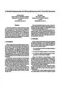
Figure 3: Hadoop DataNode logs in M45 cluster

Hadoop is an open-source implementation of MapReduce and the Google File System architecture [4, 7]. We looked at logs from two different Hadoop deployments: a 15-node Hadoop cluster at our institution and the 4000node “M45” cluster operated by Yahoo!, inc and used by academics at many different institutions. We show how our visualization brings out important characteristics of Hadoop’s logging in a workload-independent way, while also highlighting interesting and relevant differences between the two sites. Hadoop is a large, mature, well-engineered system with extensive logging. Hadoop logs are identifierrich, and most identifiers are easily identified lexically. For instance, all job IDs match the regular expression job [0-9]+ [0-9]+ . Other identifiers are similar, consisting of a sigil specifying the identifier class, followed by several numeric fields, separated by underscores. Hadoop’s identifiers make heavy use of subsumption— task a b is a task required by job a, and attempt a b c is an attempt by a particular node to perform task task a b. Figure 3 shows the identifier graph for a Hadoop DataNode in the M45 cluster. (DataNodes are the worker nodes for the HDFS filesystem.) This graph illustrates several ways that the identifier graph characterizes logs. One message type, number 2, is both commonly occurring and ubiquitous for blocks. These messages are block verification reports, which automatically generated periodically for every block, making them both ubiquitous and common. More interestingly, no other message type is particularly common or ubiquitous: all other message types are both rare (boxes drawn with thin blue lines) and also not ubiquitous (lines to “Block” drawn thin). This is a clue that we are seeing verification reports for blocks without having seen either a read or a write for them.

Analysis

As discussed in the introduction and observed in [10, 22], application logs often have the structure of a set of concurrent state machines, with a state machine for each program component; messages are logged on state transitions. Our identifier graph is approximately the dual of these state machine graphs: transitions in the state machine (messages) become nodes in the identifier graph. States in the state machine correspond to edges in the identifier graph, since each edge indicates that the state machine (identifier node) could be in a particular state (message node). Our representation goes farther, however, since it incorporates the messages that correspond to transitions in multiple linked state machines. The connectedness of the graph corresponds to the complexity of the underlying logging. A log message describing an interaction between components will appear on the graph as a node with multiple edges. The number of messages linked to an identifier indicates how much detail the logging gives about the activities of that kind of entity (the number of state machine states, perhaps). The number of identifier classes gives a sense how many different aspects of program behavior the logging records.

3

5)67&*+89

:%;(

4

Characterizing and comparing logs

In the introduction, we set two goals: characterizing the logs from a program and finding omissions or weaknesses. In this section, we describe how our graphs achieve the first of those goals: characterizing logs in ways that facilitate comparison. 4

9&:(

7&8( !,

+.

!2

)3 )1

.*

36

* !-

*-

7#'18&32

!5

)6

6 !4

!3

)/

*

*6

)-

-+ !

5

+,,-./,

)0 +!

*)

**

2 3

0112341

%&'(

1!

7-8#9-:;

**

)*

!

+*

"#$ )*

10

30

4

%&'( -!

+ 61

66 "#,+2#

68

64

! 6-

"#$%&'()#*"+, -0

-/

-!

Figure 6: SCADS identifier graph. Larger connected components are high-level actions, smaller components are low-level. several kinds of log analysis: it makes it impossible to compute metrics like average task run time unambiguously from the logs. The SCADS developers confirmed this as a bug, and they intend to add time-stamps or some other additional disambiguating information to their action identifiers. Note that a per-message timestamp is insufficient here, because several concurrent actions can take place with the same participants. The statement graph also illustrates a second problem with the SCADS logs. Even though there is a welldefined correspondence between high- and low-level actions, the logs do not reflect this. No messages link lowand high-level actions. In our taxonomy above, this qualifies as an absence of expected identifiers. This is problematic because if an unexpected low-level action appears in the logs, there is no straightforward way to find out what high-level task spawned it. Likewise, there is no convenient way to see which low-level actions were spawned by a given high-level task. The SCADS developers hope to fix this problem in their next release by explicitly logging the dependence between a low-level action and the high-level action that caused it.

4.2

Chukwa

Chukwa is an open source log collection and processing framework, currently in production use at several sites [2]. It is a fairly substantial distributed system and produces its own console logs describing what data sources are being monitored and the flow of data through 6

the system. In Chukwa, data is produced by system components called adaptors. Like many open-source efforts, Chukwa is the work of several developers, each of whom instrumented the portion of the system they were working on. As a result, Chukwa’s logging uses several different schemes for referring to adaptors. In some places, adaptors are referred to by an ID string, and in other places by their functional description. In the first version of Chukwa we looked at, the mapping between these two naming styles was never explicitly recorded: there was no way, given the logs, to know the function of an adaptor, given the ID.

+0 +,

/8

7'3& +!

9:;

-.

+