A Greedy, Graph-Based Algorithm for the Alignment of Multiple ...
Recommend Documents
Jun 7, 2012 - extend greedy algorithms to the class of models that can only/best be .... kinds of objects cannot be compared in an âapples to applesâ way, which ... results in an increase in the loss; the corresponding cost is the same weighting
Abstract. We consider a branch-and-cut approach for solving the multiple sequence align- ment problem, which is a central problem in computational biology.
HSA runs in four steps: Step 1: (Initialization) We start by building a directed graph from the input proteins as follows. Each residue maps to a vertex in the graph.
Jun 9, 2014 - GASOLINE has been developed in Java, and is available, along ... Fondo Europeo per lo Sviluppo Regionale (PO-FESR) 2007â2013), Linea di intervento ...... (PDF). Acknowledgments. We thank Professor Roded Sharan and ...
Easy to implement and fast to converge in early iterations, the FW algorithm has .... power and storage capacity, RAM usage of path-based algorithms is no ...
from a kernel-induced dictionary. Vincent and Bengio (2002) compared the performance of KMP with. SVM and RBF networks on several real world data sets.
words according to a static dictionary such that the original text is encoded by a .... dictionaries a small gap remains towards the upper bound due to asymptotic ...
Available online at www.prace-ri.eu. Partnership for Advanced Computing in Europe. 1. Massively Parallel Algorithm for Multiple Sequence Alignment. Based on ...
system design and grid computing. S. Kuppuswami obtained his BE and MSc Engg. in Electronics from the. University of Madras. He also received his Doctorate ...
An ant colony algorithm for multiple sequence alignment in bioinformatics. Jonathan Moss and Colin G. Johnson â. âComputing Laboratory University of Kent at ...
Jun 7, 2017 - software package (http://alurulab.cc.gatech.edu/phylo). We use X and Y .... All experiments are preformed in an Apple Macbook. Pro (Mid-2012 ...
multiple access (STDMA) under the physical interference model has been shown to be an NP-hard problem [5]. Thus, scheduling algorithms often rely on ...
Nov 26, 2013 - the best experimental design, randomly selected groups can only be randomly different on ... Journal of Statistical Software â Code Snippets. 3. 2. ..... 10 repsample: Representative Sampling in Stata. Let us assume we wish to ...
aindustrial and Systems Engineering Department, University of Florida, ... bOperations Research Center, Massachusetts Institute of Technology, ... cDepartment of Computer Science, State University of New York, Stony Brook, NY 11 794, USA.
S. J. DILWORTH, N. J. KALTON, DENKA KUTZAROVA, AND V. N.. TEMLYAKOV ...... [5] R. C. James, Bases and reflexivity of Banach spaces, Ann. of Math. 52.
Jul 11, 2014 - We describe our participation in the short text track of the. Entity Recognition and ... (ERD) challenge is to recognize entity mentions in a given.
ements of the kernel matrix (Drineas and Mahoney,. 2005), or the ... 10 15 20 25. 0. 50. 100. 150. 200. Reuters-21578, k=l l/n (%). R u n tim e. (se co n d s). 5.
Jul 27, 2010 - rected graph, where each voxel is a vertex and each pair of neighboring voxels is .... shot, with uniform density (one fiber bundle per voxel) and.
For a kernel matrix K â RpÃp: ËK a low rank approximation of K. ËKk the best rank-k approximation of K ob- tained using singular value decomposition. ËKS.
almost true maximum approximation âgainâ is considered, respectively. An extensive survey of greedy ...... VKOGA aâpost. bnd. Fig. 3 Left: Relative errors on ...
Nov 5, 2017 - Claremont, CA 91711. Rachel Grotheer. Center for Data, Mathematical, and Computational Sciences. Goucher College. Baltimore, MD 21204.
Jul 23, 2004 - Abstract. In the Minimum Common String Partition problem (MCSP) we are given two strings on input, and we wish to partition them into the ...
F. D. J. Dunstan, A. W. Ingleton, and D. J. A. Welsh [3] introduced the concept of a supermatroid defined on a poset in 1972 as a generalization of a matroid.
(gradMP), to solve a general sparsity-constrained optimization. .... RSS, which has been the essential tools to show the
A Greedy, Graph-Based Algorithm for the Alignment of Multiple ...
Jan 6, 2011 - graph-based alignment algorithm will be explained, followed by the development ..... As a consequence of the max-flow, min-cut theorem (Elias.
Bioinformatics Advance Access published January 6, 2011
A Greedy, Graph-Based Algorithm for the Alignment of Multiple Homologous Gene Lists Jan Fostier 1,∗ , Sebastian Proost 2,3,∗ , Bart Dhoedt 1 , Yvan Saeys 2,3 , Piet Demeester 1 , Yves Van de Peer 2,3,† and Klaas Vandepoele 2,3 1
Department of Information Technology (INTEC), Ghent University, Gaston Crommenlaan 8, bus 201, Ghent, Belgium. 2 Department of Plant Systems Biology, VIB, Technologiepark 927, Ghent, Belgium. 3 Department of Plant Biotechnology and Genetics, Ghent University, Technologiepark 927, Ghent, Belgium.
ABSTRACT Motivation: Many comparative genomics studies rely on the correct identification of homologous genomic regions using accurate alignment tools. In such case, the alphabet of the input sequences consists of complete genes, rather than nucleotides or amino acids. As optimal multiple sequence alignment is computationally impractical, a progressive alignment strategy is often employed. However, such an approach is susceptible to the propagation of alignment errors in early pairwise alignment steps, especially when dealing with strongly diverged genomic regions. In this paper, we present a novel accurate and efficient greedy, graph-based algorithm for the alignment of multiple homologous genomic segments, represented as ordered gene lists. Results: Based on provable properties of the graph structure, several heuristics are developed to resolve local alignment conflicts that occur due to gene duplication and/or rearrangement events on the different genomic segments. The performance of the algorithm is assessed by comparing the alignment results of homologous genomic segments in Arabidopsis thaliana to those obtained by using both a progressive alignment method and an earlier graph-based implementation. Especially for datasets that contain strongly diverged segments, the proposed method achieves a substantially higher alignment accuracy, and proves to be sufficiently fast for large datasets including a few dozens of eukaryotic genomes. Availability: http://bioinformatics.psb.ugent.be/software. The algorithm is implemented as a part of the i-ADHoRe 3.0 package. Contact: [email protected]
1 INTRODUCTION In the past decades, considerable effort has been devoted to the development of algorithms for the alignment of biological sequences at the nucleotide or amino acid level. Using dynamic programming techniques, optimal pairwise global (Needleman and Wunsch, 1970) ∗ Contributed † To
equally whom correspondence should be addressed
and local (Smith and Waterman, 1981) alignments can be obtained in O(l2 ) time, where l denotes the length of the sequences. A straightforward extension of these algorithms to N > 2 sequences results in a computational complexity of O(lN ), which renders the handling of sequences of realistic length impractical. Therefore, most Multiple Sequence Alignment (MSA) tools are based on progressive alignment, in which N sequences are aligned through N −1 applications of a pairwise alignment algorithm, usually guided by a tree which determines the order in which the sequences are combined. Many MSA tools that build on this principle have been implemented such as the well-known programs CLUSTAL(W) (Higgins and Sharp, 1988; Thompson et al., 1994), T-COFFEE (Notredame et al., 1998), MUSCLE (Edgar, 2004) and MAFFT (Katoh et al., 2002). Almost without exception, MSA tools target the alignment of amino acid or nucleotide sequences. In this paper, we focus on the alignment of multiple, mutually homologous (i.e. derived from a common ancestor) genomic segments, represented as gene lists. This means that the alphabet of the input sequences consists of individual genes, rather than nucleotides or amino acids. Similarly to MSA at the nucleotide or amino acid level, the goal is to align homologous genes, i.e. place genes that belong to the same gene family in the same column. The homology relationships between the individual genes have been established in a pre-processing step using sequence similarity searches and protein clustering (Kuzniar et al., 2008). Whereas ancestral gene order reconstruction (see e.g. Sankoff and Blanchette, 1998) starts from homologous genomic segments to infer ancestral genome states and quantify genome dynamics, the objective of our graph-based approach is to create accurate alignments of homologous segments, in order to facilitate the detection of additional homologous genomic segments. The multiple sequence alignment of gene lists differs significantly from the alignment of sequences at the nucleotide or amino acid level. First, the size of the alphabet of different nucleotides (four) or amino acids (twenty) is much smaller than the typical number of different gene families that occur in the genome of an organism. This means that a certain gene only has a very limited number of homologous genes in other gene lists. Second, through evolution, nucleotide and amino acid sequences mainly undergo
Downloaded from bioinformatics.oxfordjournals.org at University of Ghent on January 12, 2011
Associate Editor: Prof. Martin Bishop
2
Fig. 1. Example of the graph-based aligner for three simple gene lists. (a)-(e) Basic alignment algorithm. The active nodes are contained in the dashed rectangle. Note that the basic alignment procedure is ‘stalled’ in (c) and that two conflicting links have to be removed first (d), to allow the aligner to continue. (f) Resulting alignment.
(called GG2), that builds on the original GG-aligner. First, the basic graph-based alignment algorithm will be explained, followed by the development of a heuristic to resolve consistency problems in this graph, so-called conflicts. In later sections, we demonstrate that the new GG2-aligner outperforms both the pNW method and the original GG-aligner in terms of alignment accuracy. The new GG2aligner has been implemented in the latest 3.0 version of i-ADHoRe and its C++ source code can be downloaded for academic purposes (http://bioinformatics.psb.ugent.be/software).
2 ALGORITHM 2.1 Graph structure Consider a set of N unaligned genomic segments that are known to be mutually homologous. Each of the segments is represented by an ordered list that contains the genes in the same order as they appear on the corresponding segment. The number of genes in the ith list is denoted by li . Every gene in a list is homologous to zero or more genes in other lists. Although tandem duplicated genes on a genomic segment are largely filtered from the input by i-ADHoRe (see Section 3.1), their presence within the unaligned segments does not interfere with the alignment procedure. The gene lists can be represented together as a single graph G(V, E, w) as follows. First, the genes are represented by vertices (or nodes) V . The j th node (j = 1 . . . li ) on the ith gene list (i = 1 . . . N ) is referred to by ni,j . The functions seg(.) and ind(.) return the gene list and the position index of a node respectively, i.e. seg(ni,j ) = i and ind(ni,j ) = j. Second, consecutive genes on a segment (i.e. ni,j and ni,j+1 ) are connected through a directed arc or so-called edge pointed towards the gene with the highest index (the right-most gene). These directed edges simply connect the genes on a segment in a linear fashion. Finally, homologous genes located on different segments are connected through an undirected arc or so-called link. No links are created between homologous genes on the same segment (tandem duplicates). A weight w can be attributed to each link. The higher this weight is taken, the more likely it is that the two nodes connected by this link, will show up in the same column in the final alignment. This will be explained in later sections. The graph corresponds to the ‘extended alignment graph’ as
Downloaded from bioinformatics.oxfordjournals.org at University of Ghent on January 12, 2011
character substitutions, whereas chromosomes mainly undergo gene loss/insertion, inversion and other types of rearrangements (e.g. reciprocal translocation). These two major differences allow for the development of a graph-based alignment approach, which will be demonstrated to have a higher accuracy than a progressive approach, in terms of the number of correctly aligned homologous genes. We propose an algorithm similar to the so-called segment-based alignment approach that is used in e.g. DIALIGN (Morgenstern, 1999). The first step in DIALIGN consists of the identification of corresponding gap-free local alignments or ‘fragments’ between pairs of sequences. The alignment of some of these fragments can prohibit the alignment of others. Finding the largest (weighted) subset of fragments that can be incorporated into a multiple alignment is a difficult task, often referred to as the consistency problem (Corel et al., 2010). In the context of the gene list alignment problem, the ‘fragments’ correspond to homologous genes. The consistency problem then is to find the maximal number of homologous genes that can be included in a multiple alignment. Optimal solution methods to this consistency problem exist (Lenhof et al., 1999), but are NPhard and therefore in general computationally impractical. Here, fast heuristic methods are developed to remove inconsistent or conflicting homology relationships between genes, from a graph-theoretic perspective. Similar ideas have been developed by Pitschi et al., 2010. The proposed alignment algorithm is part of the i-ADHoRe (iterative Automatic Detection of Homologous Regions) software (Simillion et al., 2004, 2008), a map-based method to detect homologous genomic segments within or between the genomes of related organisms. Rather than identifying primary sequence similarity, map-based methods look for statistically significant conservation of gene content and gene order (collinearity). One of the key features of i-ADHoRe is the capability to uncover segmental homology, even between highly diverged segments. When two homologous segments have been identified, a so-called profile is constructed by aligning both segments, hence combining the gene order and content of both homologous segments. This genomic profile can then be used by i-ADHoRe as a more sensitive probe to scan the genome, in order to identify additional homologous segments (Simillion et al., 2004). This iterative process of alignment and detection continues, until no additional statistically significant genomic segments can be found. It is clear that a high-quality alignment of the homologous gene lists within a profile is imperative for a sensitive detection of additional homologous genomic segments within the i-ADHoRe software. The original i-ADHoRe (Simillion et al., 2004) implementation relied on profile construction using a progressive application of the Needleman-Wunsch (pNW) aligner. Especially when dealing with strongly diverged segments, one of the biggest problems with the pNW method is that erroneous alignment decisions in early pairwise steps propagate to the final alignment, causing the alignment quality to degrade significantly when more segments are added. This problem was already partially addressed in i-ADHoRe 2.0, through the introduction of a greedy, graph-based (GG) aligner (Simillion et al., 2008). Rather than relying on a progressive adding of segments, the GG-aligner considers the N segments ‘simultaneously’. Although this GG-aligner has its merits compared to the pNW-aligner (e.g. it avoids the ‘once a gap, always a gap’ problem), it was unable to outperform the latter in terms of the number of correctly aligned genes. This paper introduces a new greedy, graph-based algorithm
introduced by Lenhof et al., 1999, although a slightly different terminology has been adopted here.
2.2 Basic alignment procedure
2.3 Conflicts and cycles in G The basic alignment procedure described above is straightforward, as long as no alignment conflicts are encountered. We define a conflict as a set of links that cannot be aligned, i.e. the alignment of some links in the set prohibits the alignment of other links. By the expression ‘alignment of a link’, we mean the alignment of the two nodes connected by the link. Sources for alignment conflicts are gene duplications, local inversions, translocations and false positive homology assignment between genes. In Section 2.5, we will be prove that if no alignable set S can be found among the active nodes, such a conflict is always present. Conflicts can only be resolved by removing one or more links that contribute to the conflict. This means that certain homologous genes will not be placed in the same column in the final alignment. Because the goal of the algorithm is to minimize this number of misaligned (taking the weight w of the links into account), it is imperative to carefully select which links are removed. The presence of links and edges induces an ordering of the nodes in the graph G. Consider two nodes u and v, for which a path P in G exists from u to v. In general, such a path consists of both links and edges. The latter can only be traversed in the sense indicated by their arrow, i.e. from left to right. If a path from vertex u to vertex v contains at least one edge, then the order relationship u ≺ v holds. This means that, if all links in P were to be aligned (suppose that this is possible), node u would necessarily end up in a column left to the column containing node v in the final result. We call such a path a blocking path PB with respect to to the nodes u and v, as opposed to a direct path PD , that contains only links and hence implies that nodes u and v should be aligned. This is indicated by u ∼ v. A path from node u to node v imposes a direction on the links that are part of that path. In this context, the
Fig. 2. (a) The path PB = {L2 , L3 , L4 } defines an elementary blocking path from node u to v. Similarly, PD = {L2 , L3 } is an elementary direct path between nodes x and y. The cycle CC = {L1 ∪ PB } is an elementary blocking cycle, corresponding to a minimal conflict of degree 4. Removing any link from CC will resolve the conflict. (b) The path PB = {L2 , L3 , L4 , L5 } is a blocking path from u to v, however, the path is not elementary since both links L3 and L5 originate from nodes on the same segment. Indeed, even though CC = {L1 ∪ PB } is a blocking cycle in G, the removal of e.g. L1 does not resolve the conflict. The cycle 0 = {L , L } (hence C 0 ⊂ C ) on the other hand is an elementary CC 3 4 C C 0 resolves the blocking cycle. Removing either one of the two links in CC conflict.
functions tail(.) and head(.) return the initial and terminal vertex of a such a link, respectively. This directional property of links exists only in the context of the specified path. A path P from node u to node v can unambiguously be described by only listing the links –and not the directed edges (if any)– in the order of appearance in the path, i.e. P = {Li } (i = 1 . . . p), where seg(u) = seg(tail(L1 )), ind(u) ≤ ind(tail(L1 )), seg(head(Li )) = seg(tail(Li+1 )), ind(head(Li )) ≤ ind(tail(Li+1 )), ∀i = 1 . . . p − 1, seg(v) = seg(head(Lp )) and ind(head(Lp )) ≤ ind(v). Given a link L1 between nodes u and v, an alignment conflict occurs, when there is at least one blocking path PB = {Li } (i = 2 . . . p) from u to v. Indeed, the presence of L1 implies that u ∼ v, whereas the presence of PB implies that u ≺ v, a contradiction. Clearly, it is impossible to align all links in the set {Li } (i = 1 . . . p), hence they generate a conflict. The union CC = {L1 ∪ PB } is a so-called conflicting cycle in the graph G. We define a conflicting cycle as a closed path in G that contains at least one (directed) edge. By this reasoning, one can immediately see that alignment conflicts correspond to conflicting cycles in G and vice versa. We define the number of links p in the cycle CC as the degree of the conflict. Clearly, the degree is at least two. Also, note that the link L1 does not play a special role in the conflict. Indeed, if we consider an arbitrary link Li (i = 1 . . . p) in CC , the links {Li+1 , . . . , Lp , L1 , . . . , Li−1 } also define a blocking path from node head(Li ) to node tail(Li ). As mentioned before, a conflict can only be resolved by removing one or more links that contribute to the conflict. If the removal of any link L i (i = 1 . . . p) from its corresponding cycle CC resolves all conflicts between the remaining links (i.e. there are no conflicting cycles left in CC \ {Li }), we say that the conflict is minimal. For any given cycle in the graph G, the number of links that terminate in nodes on a certain segment s is equal to the number of links that originate from nodes on the same segment s. If at most one link in the cycle originates from each segment, we call it elementary. The maximum number of links in an elementary cycle is therefore given by N . Similarly, an elementary path is defined as a path where at most one link originates from each segment. The maximum number of links in such a path is N − 1. Proposition 1: Minimal conflicts correspond to elementary conflicting cycles CC and vice versa. Proof: see supplementary data.
3
Downloaded from bioinformatics.oxfordjournals.org at University of Ghent on January 12, 2011
The basic workflow of the alignment algorithm is illustrated in Figure 1. Figure 1a depicts three simple unaligned gene lists. The undirected links are represented by a solid line, the directed edges by a dashed line. At any time, the basic alignment algorithm considers a set of N nodes, one node from each segment. These nodes are referred to as active nodes. For each segment i, the index ai refers to the active node ni,ai . At any time, all nodes on segment i, located to the left of the active node n i,ai have already been aligned, the nodes ni,j with an index j ≥ ai still have to be processed. Links that are incident to active nodes are called active links. The algorithm starts by considering the leftmost node from each segment, i.e. nodes {n1,1 , . . . , nN,1 }. If, among the N active nodes, a minimal set of nodes S = {nk,ak } can be found, for which each node in S is linked only to other nodes within S, this set can be aligned. We say that S is alignable. Note that S can be a singleton, and that more than one (disjoint) set can be found at a given time. The term minimal therefore refers to the fact that S should not be the union of two other alignable sets. Hence, all nodes within a minimal, alignable set S, correspond to genes that are homologous to each other. The next set of active nodes is obtained by incrementing the index ai for each segment i that has a node contained within one of the detected alignable sets. In other words, on those segments, the subsequent node is considered. At the corresponding position of all other segments, a gap is introduced. This is illustrated in Fig. 1a and 1b. This process continues until either the end of all segments is reached, or a so-called conflict is encountered. A conflict is immediately detected when no alignable set S can be found among the active nodes, as illustrated in Fig. 1c. Conflicts can only be resolved by removing one or more links (see Fig. 1d). This procedure will be explained in sections (2.3)-(2.6). Once a conflict has been resolved, the basic alignment procedure can be resumed (Fig. 1e). Note that aligning all segments ‘simultaneously’ differs conceptually from progressive alignment, where first two complete segments are aligned before considering a third one, and so on. Finally, the resulting alignment is obtained as shown in Figure 1f.
As an immediate consequence, the maximum degree of a minimal conflict is given by the number of segments N . The importance of the concept of minimal conflicts stems from the fact that such conflicts can be resolved by removing any link involved in the conflict. This is not the case for conflicts associated with non-elementary blocking cycles (compare e.g. the examples in Figures 2a and 2b). Also, from the proof of Proposition 1, it follows that any non-elementary conflicting cycle CC corresponds to one or more minimal conflicts, either by removing superfluous links from CC , or by decomposing CC into several elementary conflicting cycles. Therefore, in what follows, we only consider elementary paths, elementary cycles and minimal conflicts, without explicitly mentioning the terms elementary and minimal.
2.4 Conflict detection and resolution If the basic alignment procedure is stalled because of conflicts (i.e. no alignable set can be found among the active nodes), we want to determine which links are involved in these conflicts and which links are to be removed from G. For now, we only consider the active links as candidates for removal. In the next section, we will prove that this approach is indeed a valid one. Consider an active link between nodes ni,ai and nj,k , with i 6= j and k ≥ aj (with aj the index of the active node nj,aj ). For the simplicity of notation, these nodes are referred to as s and t respectively, the active link is denoted by Lst . The link Lst contributes to a conflict, if there is a blocking path PB between s and t or vice versa, between t and s. Indeed, the alignment of the link Lst (or any other direct path PD between s and t) implies the ordering s ∼ t. A blocking path PB from s to t implies s ≺ t, and similarly, a blocking path from t and s implies s t. We refer to these conflicts as st-conflicts and ts-conflicts respectively. To quantitatively investigate the number of conflicts that Lst is involved in, we want to assess to which degree s and t are connected through blocking paths. In graph theory, such problems can be addressed by solving
4
D C C SLst = fst − |fst − fts | C, fC) Since st-conflicts and ts-conflicts mutually conflict, at least min(fst ts capacity will need to be removed from G, regardless whether or not s and t C −f C | therefore denotes the minimal, net capacity are aligned. The term |fst ts D that will need to be removed from G if s and t are aligned. Similarly, f st denotes the minimal capacity that will need to be removed from G if s and t will not be aligned. Clearly, a positive score for SLst indicates that it is probably best to align s and t, whereas a negative score for SLst indicates that it is probably best to remove the link Lst from the graph. Note that if there are multiple st-paths, that these paths might be in mutual conflict. This fact is not taken into account by the link score SLst . In other C − f C | will effectively be words, there is no guarantee that the capacity |fst ts aligned, even if s and t are disconnected through direct paths. The algorithm for conflict resolution can now be described as follows. If, during the basic alignment procedure, described in Section 2.2, no alignable set S can be found among the active nodes, all active links are considered. For each of these links L, the score SL is calculated, and the link with the lowest score (i.e. the most problematic link), is removed from G. This process is repeated, until again, an alignable set S can be found among the active nodes. Figure 3 presents a simple example.
2.5 Active conflicts In this section, a refinement to the conflict resolution algorithm is developed. Consider a conflict situation in the graph G(V, E) (i.e. no alignable set S can be found among the N active nodes in G). Next, consider the subgraph G0 (V, E 0 ) ⊂ G(V, E) that only contains the active links (i.e. the links incident to the active nodes). We show that even in the reduced graph G0 (V, E 0 ), no alignable set can be found among the active nodes. Proposition 2: If, during the basic alignment procedure, no alignable set can be found among the N active nodes in the graph G(V, E), at least one conflict is present among the active links. Furthermore, no alignable set can be found among the same active nodes in the subgraph G0 (V, E 0 ). Proof: see supplementary data. Proposition 2 provides a more fundamental understanding of alignment conflicts. First, it shows that active links are indeed good candidates for removal. Indeed, even the removal of all non-active links would still not allow for the alignment of any of the active nodes. Second, it shows that if the basic alignment procedure is stalled, at least one conflict, consisting of active links, is present. Such a conflict is called an active conflict. None of the active nodes that are incident to a link in an active conflict can be aligned, as long as this conflict exists. Active conflicts are therefore high-priority conflicts that need to be resolved instantaneously.
Downloaded from bioinformatics.oxfordjournals.org at University of Ghent on January 12, 2011
Fig. 3. Example of a simple alignment conflict and its solution. In (a), (b) and (c), the link scores SL are calculated for the active links L1 , L2 and L3 (indicated by a bold line) respectively. All links have weight (and hence capacity) w = 1, the edges have unlimited capacity. The numbers near the links denote the flow/capacity of that link. The maximum flow from node C = 2 s to t through elementary blocking paths (indicated in red) is (a) f st C = 1 for link L , (c) f C = 1 for link L . In all three for link L1 , (b) fst 2 3 st C = 0. The cases, no conflicting flows are possible from node t to s, i.e. f ts D = 1, in all maximum flow from node s to t through direct paths is fst three cases. Therefore, SL1 = −1, SL2 = 0 and SL3 = 0. (d) Resulting alignment after the link with the lowest score (i.e. L1 ) is removed from G.
the well-known maximum flow problem. For a formal definition of the maximum flow problem, we refer to Ford and Fulkerson, 1962. Intuitively, the maximum flow is the largest amount of ‘flow’ (e.g. fluid or current) that can be transported between two given nodes, called source and sink respectively. Let fst be the maximum flow from node s to node t acting as the source and sink respectively. As an extra restriction, it is imposed that a valid flow can only pass through elementary paths (either blocking or direct) from s to t. The edges have unlimited flow capacity, however, the flow can only pass in the sense indicated by the direction of the edge (from left to right). The links have a capacity equal to their weight w, but impose no direction on the flow. There exist many polynomial algorithms for the solution of the maximum flow problem. This is more thoroughly discussed in the supplementary text. D be the maximum flow from s to t through direct eleSimilarly, let fst mentary paths. Note that this includes the flow through the link Lst . Then C = f −f D is the maximum flow from s to t through elementary clearly, fst st st blocking paths. As a consequence of the max-flow, min-cut theorem (Elias C is the minimum link capacity that has to be removed from G et al., 1956), fst to disconnect s and t through elementary blocking st-paths, i.e. to resolve all C can be calculated as the maximum flow through st-conflicts. Similarly, fts elementary blocking paths from t to s. We then use the following score to evaluate link Lst :
D C C SLst ,LB = fst,LB − max(fst,UB , fts,UB ).
In the case of conflicts, the active links can therefore be grouped into three categories: active links involved in at least one active conflict, active links involved in non-active conflicts and active links that are not involved in a conflict. The conflict resolution algorithm is therefore modified as follows. For each of the links L involved in at least one active conflict, calculate the score SL . The link with the lowest score is removed from G. It is easily determined whether or not an active link is involved in an active conflict, C and f C in the reduced graph G0 . If any of the two flows by calculating fst ts is nonzero, an active conflict is present. A simple example of the improved heuristic is illustrated in Figure 4. In the results section, it will be demonstrated that this approach indeed improves the alignment quality.
• RA (RAndom): a random link. • RC (Random Conflict): a random link that is involved in at least one (active or non-active) conflict.
• RAC (Random Active Conflict): a random link that is involved in at least one active conflict.
• LL (Longest Link): the link L, involved in at least one active conflict, incident to node nj,k for which (k − aj ) is maximum.
• LLBS (Lowest Lower Bound Score): the link L, involved in at least one active conflict, with the lowest lower bound score SL,LB .
• LS (Lowest Score): the link L, involved in at least one active conflict, with the lowest score SL .
2.6 Faster heuristics for conflict resolution The calculation of the maximum flow between two nodes in the graph is computationally expensive. However, upper bounds to the maximum flow can easily be derived. Given an active link Lst between source node s = ni,ai and sink node t = nj,k , one can immediately notice that the final link in a blocking st-path necessarily ends in a node nj,k0 with k 0 ≤ k. C Therefore, an upper bound to fst,UB can be found by summing the weights w(L) of all links incident to these nodes:
C fst,UB =
k X
X
w(L),
k0 =aj L∈nj,k0
with j =seg(t) and k =ind(t). Similarly, blocking ts-paths necessarily end C in the source node s and an upper bound fts,UB can therefore be established by summing the weights of the links L 6= Lst incident to s. C = fts,UB
X
w(L)
L∈ni,ai ,L6=Lst D is simply given by f D Finally, a lower bound to the direct flow fst st,LB = w(Lst ). Therefore, a lower bound to the link score is given by
3 RESULTS AND DISCUSSION 3.1 Datasets To test the performance of multiple sequence alignment tools, a number of benchmarks have been introduced for both protein sequences (such as BALiBASE (Thompson et al., 2005), OXBench (Raghava et al., 2003), PREFAB (Katoh et al., 2002) and SMART (Schultz et al., 1998)) and DNA sequences (Carroll et al., 2007). Because no similar benchmark exists to test the performance of gene list alignment tools, two ad hoc input datasets were generated by running the i-ADHoRe tool on the Arabidopsis thaliana (The Arabidopsis Genome Initiative, 2000) genome separately (dataset I) and on the Arabidopsis thaliana, Populus trichocarpa (Tuskan et al., 2006) and Vitis vinifera (Jaillon et al., 2007) genomes (dataset II). A. thaliana is a good candidate to validate the aligners and heuristics, since its genome contains both strongly diverged and more closely related homologous chromosomal regions (Van de Peer, 2004; Tang et al., 2008). Using the profile searches (see Simillion et al., 2008), the i-ADHoRe algorithm produces 921 and 7 821 sets of homologous genomic segments for datasets I and II respectively. The number of genomic segments N in these sets varies from 2 to 11
5
Downloaded from bioinformatics.oxfordjournals.org at University of Ghent on January 12, 2011
Fig. 4. Example of active conflicts and the improved heuristic. All links have weight w = 1. (a) Although all active links have an equal score (SL1 = SL2 = SL3 = 0), only links L1 and L2 are involved in an active conflict. The alignment of the upper two segments can not progress as long as this conflict exists. (b) Situation after L2 has been removed. Now, links L02 and L03 are involved in an active conflict, with scores SL0 = −2 and SL0 = 0. 2 3 (c) Final alignment after L02 has been removed.
Selecting the active link L with the lowest lower bound score SL,LB yields a much faster heuristic. Indeed, the calculation of SL,LB requires no maximum flow problems to be solved. Even though this lower bound estimation may be significantly underestimating the actual score SLst , it still provides a powerful method to select a link for removal, if we assume that the link with the lowest lower bound score is also the link with the lowest score. Taking this reasoning even a step further, the heuristic can even be further simplified, if one assumes that the sum of the weights of the links, incident to a node, is constant for all nodes, i.e. that the links are evenly distributed among the nodes. Given a link Lst between source node s = ni,ai and sink C node t = nj,k , this means that fst,UB is proportional to (k − aj ), while C C fts,UB and fst,LB are constant. This is clearly a rather rough approximation, however, it leads to the very simple and fast heuristic: select the active link incident to node nj,k for which the ‘length’ of the link (k −aj ) is maximal (the ‘longest’ link). Such a link has the most possibilities for conflicting st-paths, and is hence a good candidate for removal. We now summarize the heuristics for conflict resolution and introduce three random methods. These random methods are not of any particular interest, but it is always interesting to compare the more mathematically supported methods to random methods. Select, in the case of a conflict, among the active links, the following link for removal:
Table 1. Comparison of the number of correctly aligned homologous genes in dataset I. The scores of the random methods are averaged over 1 000 runs.
(dataset I) and from 2 to 15 (dataset II). For both datasets, the iADHoRe settings were gap size = 30, cluster gap = 35, q = 0.75 and p = 0.01. Tandem duplicates within a distance of gap size / 2 were remapped onto the representative gene with the lowest index.
3.2 Alignment accuracy To detect homologous segments, i-ADHoRe looks for statistically significant conservation of gene content and order. When two homologous segments are visualized in a dot-plot, their collinearity shows up as a ‘diagonal’. The homologous gene pairs between the two segments that are used by i-ADHoRe to detect these ‘diagonals’, are called anchors. These anchors are a subset of all homologous gene pairs between the two segments. By giving a higher weight to the links associated with anchors, they can effectively be used as an alignment guide to improve the overall alignment quality. In all simulations, the weight w of the links corresponding to anchors was set to 1, whereas the weight of the other links was set to 0.1. These other links correspond to homologous genes that are further offdiagonal, and therefore less likely to be aligned in the final result. Note that more complex weight schemes could be incorporated, possibly improving alignment results. For example, the link weights could represent the probability that two genes are truly homologous. In this work, such schemes were not investigated. The proposed greedy, graph-based aligner (GG2) is compared to both a progressive application of the Needleman-Wunsch method (pNW) and the original greedy, graph-based aligner (GG). The pNW-aligner first performs a pairwise alignment of the two genomic segments that share the most anchor points, i.e. the two most closely related segments. Subsequently, a third segment is added to this intermediate result and so on. It should be noted that more advanced improvements to this basic progressive approach have been implemented, e.g. by using a guide tree to determine the order in which the segments are added (Thompson et al., 1994), or by incorporating consistency-objective functions (Notredame et al., 2000). The original graph-based GG-aligner relies on the same ‘basic alignment procedure’ as the GG2-aligner, however, conflicts are handled in a more primitive fashion. In short, based on the number of links and their lengths (cfr. Section 2.6), the GG-aligner calculates a score for each active node (as opposed to for each active link in the GG2-aligner). Instead of removing a single link, the GG-aligners
6
removes all links incident to the active node with the lowest score. In the GG-aligner’s heuristic, no thorough analysis of conflicting paths or links is conducted. In Table 1, the number of correctly aligned homologous genes for the profiles generated by the different aligners are compared for dataset I. We consider two homologous genes to be correctly aligned if they are placed in the same column in the final result. This omits the need for a reference alignment. The numbers in Table 1 therefore correspond to the sum-of-pairs metric. Each row shows the accumulated sum-of-pairs scores for all input sets with a specified number of segments N (N = 2 . . . 11). The final row represents the sum-of-pairs over all profiles, and can therefore be seen as a quality benchmark for the complete dataset. First, it is immediately clear that all random methods perform significantly worse than the more mathematically supported heuristics. The score of the RA-aligner is an indication of the number of homologous genes that can be aligned ‘for free’ by the basic alignment procedure. The fact that this score is rather high means that a fairly large number of links is not involved in any conflict. Indeed, if for example all input segments were identical (perfect collinearity and hence no conflicts), all methods would produce identical (and optimal) results. When comparing the numbers of the other aligners, it is important to keep this consideration in mind. The RCaligner improves the RA score, by making sure that no active links are removed that do not contribute to any conflict. Interestingly, the alignment score is again significantly improved by using the RACaligner, which selects a random active link, involved in at least one active conflict. This provides experimental evidence for the observations made in Section 2.5, i.e. that active conflicts are high-priority conflicts. Note that in the case of a conflict for N = 2, all active links are necessarily involved in an active conflict. Therefore, the RA, RC and RAC heuristics perform equally well for N = 2. The LL, LLBS and LS heuristics strongly outperform both the random methods and the original GG-aligner, and, albeit to a somewhat lesser extent, also the pNW-method. Unsurprisingly, the pNW-aligner is best for N = 2, since it produces optimal results. The LL, LLBS and LS methods however, also obtain close to optimal results. For larger N , the relative difference in score between pNW on the one hand and LL, LLBS and LS one the other hand increases. This is to be expected: erroneous alignment decisions in
Downloaded from bioinformatics.oxfordjournals.org at University of Ghent on January 12, 2011
N 2 3 4 5 6 7 8 9 10 11 P
# input sets 447 169 119 49 41 39 24 16 13 4 921
3.3 Program runtime A comparison for the alignment times of the different heuristic methods can be found in Table 2 for the larger dataset II. Except for the LS heuristic, the total alignment times are very low. The unfavorable time complexity of the LS heuristic prohibits the alignment of sequences with larger N . In practice, when N > 10, the CPU time for the LS method rapidly increases. In i-ADHoRe, we therefore offer the LLBS heuristic by default. Experiments on an extremely large dataset consisting of dozens of eukaryotic species (Hubbard et al., 2009) have shown that this method can easily handle N=50, enough for most practical problems. A detailed analysis of the computational complexity of the algorithm is given in supplementary data.
Table 2. Comparison of alignment scores and runtimes for dataset II.
respectively, whereas i-ADHoRe detects 90.3% and 25.8% respectively. In agreement with the yeast results reported by DRIMM, including a more ancestral genome lacking a recent whole-genome duplication (e.g. Vitis in dataset II) serves as a reference backbone to identify and align highly diverged Arabidopsis genomic segments (Van de Peer et al., 2009).
4 CONCLUSION We have developed a greedy, graph-based algorithm for the alignment of multiple, homologous gene lists. Several properties of conflicts within the alignment graph have been derived and proved. Three heuristics for conflict resolution were developed on these theoretical grounds, and have been demonstrated to be able to outperform an older graph-based algorithm and a progressive approach in terms of alignment accuracy. As is often the case, a trade-off between computational requirements and alignment accuracy can be observed. The algorithm has been implemented in the latest version of i-ADHore 3.0. Funding: This project is funded by the Research FoundationFlanders and the Belgian Federal Science Policy Office: IUAP P6/25 (BioMaGNet). We acknowledge the support of Ghent University (Multidisciplinary Research Partnership “Bioinformatics: from nucleotides to networks”). KV and YS are Postdoctoral Fellows of the Research Foundation-Flanders (FWO). SP thanks the Institute for the Promotion of Innovation by Science and Technology in Flanders for a predoctoral fellowship.
3.4 Comparison of i-ADHoRe to related tools The GG2-aligner is an important component of i-ADHoRe, which detects evolutionary related genomic regions within or between related species through sensitive iterative profile searches. In contrast to this approach, CYNTENATOR (R¨odelsperger and Dieterich, 2010) and the method described by Fritzsch et al. (2006) compute multiple gene order alignments progressively using initial pairwise alignments and a guide tree. DRIMM-Synteny (Pham and Pevzner, 2010) detects non-overlapping synteny blocks to perform rearrangement analysis in duplicated genomes and reconstruct ancestral genomes. Although our method does not infer likely evolutionary paths of genome evolution events, the application of the profile search on the Arabidopsis genome (dataset I) identifies a much larger fraction of the genome in duplicated blocks, compared to DRIMM. Pham and Pevzner report fractions of 66% and 8% in duplicated blocks with a multiplicity of at least two and at least four
REFERENCES Carroll, H., Beckstead, W., O’Connor, T., Ebbert, M., Clement, M., Snell, Q., and Mcclellan, D. (2007). Dna reference alignment benchmarks based on tertiary structure of encoded proteins. Bioinformatics, 23(19), 2648–2649. Corel, E., Pitschi, F., and Morgenstern, B. (2010). A min-cut algorithm for the consistency problem in multiple sequence alignment. Bioinformatics, 26(8), 1015–1021. Edgar, R. C. (2004). Muscle: multiple sequence alignment with high accuracy and high throughput. Nucleic acids research, 32(5), 1792–1797. Elias, P., Feinstein, A., and Shannon, C. (1956). A note on the maximum flow through a network. Information Theory, IRE Transactions on, 2(4), 117–119. Ford, L. and Fulkerson, D. (1962). Flows in networks. Princeton University Press, Princeton, NJ. Fritzsch, G., Schlegel, M., and Stadler, P. F. (2006). Alignments of mitochondrial genome arrangements: Applications to metazoan phylogeny. Journal of Theoretical Biology, 240, 511–520.
7
Downloaded from bioinformatics.oxfordjournals.org at University of Ghent on January 12, 2011
early pairwise steps of the pNW-aligner propagate when more segments are added. The graph-based methods are more robust in the sense that they take the links on all segments into consideration. For higher N , the difference in score between LS and pNW is larger than 10%. In total, the LS-method is able to align 846 (4.4%) more homologous genes than the pNW methods. An alignment example of six homologous genomic segments in the A. thaliana genome as produced by the pNW and the LS heuristic is given in supplementary Fig. 3. The difference in alignment quality between the LL, LLBS and LS heuristics is rather modest, however, it can be observed that LL < LLBS < LS, for nearly all N . Despite the simplicity of the LL heuristic, this method still performs remarkably well, and even outperforms the pNW method on this dataset. The biggest difference between these methods lies in the alignment speed. This will be discussed in more detail in the next section. It is important to mention that the relative difference in alignment quality between the pNW on the one hand and the LL, LLBS and LS heuristics associated with the GG2-aligner on the other hand, decreases for datasets that consist of genomic segments that are less diverged. For instance, Table 2 lists the alignment scores for dataset II. Even though the ranking of the different alignment methods remains the same, the relative difference in alignment score is smaller. This is due to the fact that relatively fewer alignment conflicts exists in this dataset, which can be seen from the high score of the random aligners.
8
Sankoff, D. and Blanchette, M. (1998). Multiple genome rearrangement and breakpoint phylogeny. Journal of Computational Biology, 5, 555–570. Schultz, J., Milpetz, F., Bork, P., and Ponting, C. P. (1998). Smart, a simple modular architecture research tool: Identification of signaling domains. Proceedings of the National Academy of Sciences of the United States of America, 95(11), 5857–5864. Simillion, C., Vandepoele, K., Saeys, Y., and Van de Peer, Y. (2004). Building genomic profiles for uncovering segmental homology in the twilight zone. Genome research, 14(6), 1095–1106. Simillion, C., Janssens, K., Sterck, L., and Van de Peer, Y. (2008). i-ADHoRe 2.0: an improved tool to detect degenerated genomic homology using genomic profiles. Bioinformatics (Oxford, England), 24(1), 127–128. Smith, T. F. and Waterman, M. S. (1981). Identification of common molecular subsequences. Journal of molecular biology, 147(1), 195–197. Tang, H., Bowers, J. E., Wang, X., Ming, R., Alam, M., and Paterson, A. H. (2008). Synteny and collinearity in plant genomes. Science, 320(5875), 486–488. The Arabidopsis Genome Initiative (2000). Analysis of the genome sequence of the flowering plant Arabidopsis thaliana. Nature, 408(6814), 796–815. Thompson, J. D., Higgins, D. G., and Gibson, T. J. (1994). Clustal w: improving the sensitivity of progressive multiple sequence alignment through sequence weighting, position-specific gap penalties and weight matrix choice. Nucleic acids research, 22(22), 4673–4680. Thompson, J. D., Koehl, P., Ripp, R., and Poch, O. (2005). Balibase 3.0: latest developments of the multiple sequence alignment benchmark. Proteins, 61(1), 127–136. Tuskan, G. A., DiFazio, S., Jansson, S., et al. (2006). The genome of black cottonwood, populus trichocarpa (torr. & gray). Science, 313(5793), 1596–1604. Van de Peer, Y. (2004). Computational approaches to unveiling ancient genome duplications. Nature Reviews Genetics, 5(10), 752–763. Van de Peer, Y., Fawcett, J. A., Proost, S., Sterck, L., and Vandepoele, K. (2009). The flowering world: a tale of duplications. Trends in Plant Science, 14(12), 680–688.
Downloaded from bioinformatics.oxfordjournals.org at University of Ghent on January 12, 2011
Higgins, D. G. and Sharp, P. M. (1988). Clustal: a package for performing multiple sequence alignment on a microcomputer. Gene, 73(1), 237–244. Hubbard, T. J. P., Aken, B. L., Ayling, S., et al. (2009). Ensembl 2009. Nucl. Acids Res., 37(suppl 1), D690–697. Jaillon, O., Aury, J.-M., et al. (2007). The grapevine genome sequence suggests ancestral hexaploidization in major angiosperm phyla. Nature, 449(7161), 463–467. Katoh, K., Misawa, K., Kuma, K.-i., and Miyata, T. (2002). Mafft: a novel method for rapid multiple sequence alignment based on fast fourier transform. Nucleic acids research, 30(14), 3059–3066. Kuzniar, A., van Ham, R. C., Pongor, S., and Leunissen, J. A. (2008). The quest for orthologs: finding the corresponding gene across genomes. Trends in genetics : TIG, 24(11), 539–551. Lenhof, H., Morgenstern, B., and Reinert, K. (1999). An exact solution for the segmentto-segment multiple sequence alignment problem. Bioinformatics, 15, 203–210. Morgenstern, B. (1999). Dialign 2: improvement of the segment-to-segment approach to multiple sequence alignment. Bioinformatics, 15(3), 211–218. Needleman, S. B. and Wunsch, C. D. (1970). A general method applicable to the search for similarities in the amino acid sequence of two proteins. Journal of molecular biology, 48(3), 443–453. Notredame, C., Holm, L., and Higgins, D. G. (1998). Coffee: an objective function for multiple sequence alignments. Bioinformatics, 14(5), 407–422. Notredame, C., Higgins, D. G., and Heringa, J. (2000). T-coffee: A novel method for fast and accurate multiple sequence alignment. Journal of molecular biology, 302(1), 205–217. Pham, S. K. and Pevzner, P. A. (2010). DRIMM-Synteny: decomposing genomes into evolutionary conserved segments. Bioinformatics, 26, 2509–2516. Pitschi, F., Devauchelle, C., and Corel, E. (2010). Automatic detection of anchor points for multiple sequence alignment. BMC bioinformatics, 11, 445+. Raghava, G. P. S., Searle, S., Audley, P., Barber, J., and Barton, G. (2003). Oxbench: A benchmark for evaluation of protein multiple sequence alignment accuracy. BMC Bioinformatics, 4(1), 47+. R¨odelsperger, C. and Dieterich, C. (2010). CYNTENATOR: progressive gene order alignment of 17 vertebrate genomes. PloS one, 5(1), e8861+.