ne of the disadvantages of a univariate monitoring scheme is that for a single .... where, is a measure of quality level, and the best quality level is 0 and the.
Quality Technology & Quantitative Management Vol. 3, No. 4, pp. 437-453, 2006
QTQM © ICAQM 2006
Multivariate Fuzzy Multinomial Control Charts Hassen Taleb1, Mohamed Limam2 and Kaoru Hirota3 1, 2 LARODEC, Institut Supérieur de gestion University of Tunis cité bouchoucha, Bardo , Tunisia 3 Interdisciplinary Graduate School of Science and Engineering, Tokyo Institute of Technology Nagatsuta, Midori-ku, Yokohama City, Japan
(Received March 2005, accepted December 2005)
______________________________________________________________________ Abstract: Two approaches for constructing control charts to monitor multivariate attribute processes when data set is presented in linguistic form are suggested. Two monitoring statistics T f2 and W 2 are
developed based on fuzzy and probability theories. The first is similar to the Hotelling’s T 2 statistic and is based on representative values of fuzzy sets. The distribution of W 2 statistic, being a linear combination of dependent chi-square variables, is derived using Satterthwaite’s approximation. Resulting multivariate control charts are compared based on the average run length (ARL). A numerical example is given to illustrate the application of the proposed multivariate control charts and the interpretation of out-of-control signals.
Keywords: Bootstrap, categorical data, fuzzy control, Satterthwaite’s approximation.
______________________________________________________________________ 1. Introduction
O
ne of the disadvantages of a univariate monitoring scheme is that for a single process, many variables may be monitored and even controlled. Multivariate quality control (MQC) methods overcome this disadvantage by monitoring several variables simultaneously. Using multivariate quality control methods, engineers and manufacturers, who monitor complex processes, may monitor the stability of their processes. With modern data-acquisition equipment and on-line computers it is now common practice to monitor several quality characteristics (QC) simultaneously rather than a single QC during production. The most common type of control charts used in a production process is the Shewhart control chart. A multivariate QCs process could be monitored by applying a univariate Shewhart control chart for each QC. If these QCs are independent of each other, this would be an adequate procedure. However, in many production processes, multivariate QCs tend to be correlated and therefore results could be misleading and difficult to interpret. The type I error and the probability of a point correctly plotting in-control are not equal to their advertised levels for the individual control charts. Thus, it would be necessary to use a multivariate control procedure, which will take into account the internal relationship of the correlated QCs. Furthermore, it will be more practical and economical to use a single multivariate control scheme rather than several univariate Shewhart control charts. Lowry and Montgomery [10] have shown that, in monitoring multivariate process quality, a multivariate control scheme has a better sensitivity than the one based on the univariate control charts. The use of multivariate control procedures to monitor production processes is
438
Taleb, Limam and Hirota
increasingly popular. This is a result of recent advances in MQC, such as multivariate cumulative sum control chart (e.g. Crosier [3] Sullivan and Jones [20], Pignatiello and Runger [15], and Hawkins[5]), multivariate exponentially weighted moving average control charts introduced and studied by Lowry et al. [9] see also Stoumbos and Sullivan [19], Arthur et al. [1]), and Hotelling’s T 2 charts (e.g. Mason et al. [13]). Also, there is an improved effectiveness of these techniques to identify the cause of an out-of-control signal (e.g. Runger [17], etc). Wierda [22] provided an excellent review and discussion of multivariate control charts. However, most articles on multivariate control charts deal with multivariate variable processes and a little work is done for multivariate attribute processes. More recently, Lu et al. [11] proposed a control chart for multivariate attribute processes in which a product unit can be classified only as either conforming or nonconforming by each of the monitored QCs. In many cases, binary classification cannot be appropriate. In fact, quality of a product does not change abruptly from perfect to worthless. Thus, there is a need for intermediate assessments, and QCs such as appearance, softness and colour, that cannot be expressed numerically, are associated with linguistic terms such as very good, good, medium, poor,...etc. In the case of monitoring p, p = 1, 2,..., multinomial QCs, the multivariate control chart proposed by Lu et al. [11] cannot be applied. The ambiguity of linguistic variables can be analyzed with fuzzy set theory, see Zadeh [23]. In the case of p = 1 , a univariate control chart is used to control a multinomial process. Marcucci [12], Raz and Wang [16], Taleb and Limam [21] have introduced and discussed the construction of such control charts using both probability and fuzzy theory. Laviolette et al. [8] compared fuzzy and probability approach for construction of control charts for linguistic data. They suggest the superiority of the probability approach based on a simpler computational implementation. Their comparison was criticized by Kandel et al. [6], where they disagree with Laviolette et al. [8] because the comparison of the two approaches is biased. In this article the case of monitoring more than one multinomial QCs is introduced. Construction of control charts for such multivariate attribute processes is analyzed using fuzzy sets and probability theories. The framework for the proposed multivariate fuzzy chart is presented in Section 2. Multivariate probability control chart is discussed in Section 3. A numerical example is given in Section 4 to illustrate and compare the proposed approaches.
2. Fuzzy Multivariate Control Chart 2.1. Framework for the Fuzzy Approach Suppose that p related attribute QCs, c1 ,..., c p , are controlled jointly. Each QC c j , j = 1,..., p; is characterized by q j categories, or linguistic terms, which are described by fuzzy subsets. Each of these fuzzy subsets is associated with a membership function. Then, using a fuzzy transformation method each linguistic term is converted into a representative value.
Linguistic variable c j is not expressed as a numerical value, but rather as a certain word or phrase. And in fuzzy set theory, it is represented by "term set" T (c j ) . In addition, each term c jh , h = 1,..., q j , in term set T (c j ) , is characterized by a membership function µ jh ( x ) , where, x is a measure of quality level, and the best quality level is 0 and the
Multivariate Fuzzy Multinomial Control Charts
439
worst 1. It is a basic variable standardized on the interval [0,1] . Several methods for developing and selecting membership functions have appeared in the literature essentially based on statistical data (Civilnar and Trussell [2]) and ranking (Zadeh [24]). To plot easily sample characteristic values and to maintain the basic form of multivariate control charts, fuzzy subsets associated with linguistic terms in each term set should be converted into scalar values. These values are called representative values. There are four transformation methods: fuzzy median, fuzzy mode, α -level fuzzy midrange and the fuzzy average, see Raz and Wang [16]. However there is no theoretical backup for choosing one transformation method. In this chapter fuzzy median is adopted for the ease of its computation. Let there be q j linguistic variables on the term set c j , and let them be c jh , h = 1,..., q j . Let the fuzzy set for each linguistic variable be F jh which is characterized by the membership function µ jh . A sample A from n observations is then expressed by:
{{
} {
}}
A = ( F11 , n11 ),..., ( F1q1 , n1q1 ) ;...; ( F p1 , n p1 ),..., ( F pq p , n pq p ) , where n jh is the number of observations classified by linguistic variable c jh . Using fuzzy arithmetic, each QC c j is then associated with only one fuzzy subset in the following way:
Fj =
1 qj ∑ n jh F jh . n h =1
(1)
The sample A is now expressed by:
A = { F1 ,..., Fp } . Then, each fuzzy subset F j is transformed into its representative value using fuzzy median transformation method. Kaufmann and Gupta [7] showed that the multiplication of a triangular fuzzy number (TFN) T by a real number k is also a TFN. The addition of two TFN T and S is shown to be a TFN. Then a linear combination of TFN gives a TFN. For example if T and S are represented by triplets (t1 , t 2 , t3 ) and (s1 , s2 , s3 ) respectively, then a linear combination C = k1T + k 2S should be represented by triplet (k1t1 + k2 s1 , k1t 2 + k2 s2 , k1t3 + k2 s3 ) . By assuming that fuzzy variables F jh are TFNs, hence, each fuzzy number F j is also a TFN and can be written as (a1 j , a2 j , a3 j ) and its representative value is ⎧ (a3 j − a1 j )(a3 j − a2 j ) a3 j + a1 j , , for a2 j < ⎪a3 j − ⎪ 2 2 Rj = ⎨ (a3 j − a1 j )(a2 j − a1 j ) a3 j + a1 j ⎪ , for a2 j > . ⎪a1 j + 2 2 ⎩
(2)
The sample A from n observations is now expressed by the vector RA = ( RA1 ,..., RAp )′ .
(3)
440
Taleb, Limam and Hirota
Data from m samples can be expressed as: ⎛ R11 R12 ⎜ R R22 R = ⎜⎜ 21 # # ⎜ ⎜ Rm1 " ⎝
" R1 p ⎞ ⎟ " # ⎟ , % # ⎟ ⎟ " Rmp ⎟⎠
where Rij is the representative value of fuzzy number F j in the sample i . The procedure requires computing the representative values of fuzzy subsets F j , from a sample of size n . The set of representative values of the p QCs is represented by the (px1) vector in Equation (3). The test statistic being plotted on the control chart for each sample is T 2 = ( R − µ )′Σ −1 ( R − µ ),
(4)
where µ ′ = [ µ1 ,..., µ p ] is the vector of in-control means for each QC and Σ is the covariance matrix of QCs. 2.2. Estimation of Parameters µ and Σ Parameters µ and Σ should be estimated from the analysis of preliminary samples of size n , taken when the process is assumed to be in-control. Suppose that m such samples are available. The sample representative values are obtained using Equation (2). The (px1) vector of means are given by: R = ( R1 ,..., R p ), where R j = m1 ∑ im=1 Rij , and Rij is the representative value of the fuzzy subset associated with the i th sample on the j th QC. The variances of these representative values are given by: S 2j =
1 m 2 ∑ ( Rij − R j ) , m − 1 i =1
and the covariance between the j th QC and the h th QC is S jh =
1 m ∑ ( Rij − R j )( Rih − Rh ), for j ≠ h. m − 1 i =1
(5)
The p×p sample covariance matrix S is then expressed as: ⎛ S12 S12 ⎜ ⎜ S21 S 22 S =⎜ # ⎜ # ⎜S " ⎝ p1
" S1 p ⎞ ⎟ " # ⎟ ⎟. % # ⎟ " S p2 ⎟⎠
The sample covariance matrix S and the sample mean vector R are the estimates of Σ and µ , respectively, when the process is in-control.
Multivariate Fuzzy Multinomial Control Charts
2.3. The Fuzzy
T f2
441
Control Chart
Once data are collected from the stable phase of a process, they can be used to set control limits for future observed sample means. The covariance matrix S and the vector R are used to estimate Σ and µ respectively. If µ and Σ are replaced by R and S then, the statistic given in Equation (4) becomes T f2 = ( R − R )′S −1 ( R − R ).
(6)
It is important to note that the fuzzy approach consists in using the fuzzy median to transform linguistic data into measurable data. The control chart used is the traditional T 2 control chart. However, the two control charts have different characteristics. Although, under normality, the distribution of Hotelling’s T 2 statistic is known and the control limits can easily be determined, the T f2 distribution cannot be identified directly. To set control limits in the new control chart, the distribution of T f2 must be determined. However, the normality assumption does not hold for the distribution of representative value and then, the distribution of T f2 is difficult to determine directly. Now with modern computing power, although still need to rely on asymptotic theory to estimate the distribution of a statistic, resampling methods like bootstrap and jackknife return inferential results for either normal or non normal distributions. Resampling techniques such as the bootstrap and jackknife provide estimates of the standard error, confidence intervals, and distributions for any statistic. In the bootstrap, for example, B new samples, each of the same size as the observed data, are drawn with replacement from the observed data. The statistic is calculated for each new set of data, yielding a bootstrap distribution for the statistic. Steps needed to construct a T f2 control chart are as follows: Step 1: Calculate R and S −1 from available empirical observations. Step 2: Draw with replacement, from the observation data, B new samples of the same size. Step 3: Compute the statistic T fi2 = ( Ri − R )′S −1 ( Ri − R ) for each new sample i , i = 1,..., B. Step 4: Set the upper control limit such as the false alarm rate will be equal to a predefined value. 2.4. Interpreting Out-of-Control Signals The difficulty of interpreting out-of-control signals on a multivariate variable control charts has been discussed by Mason et al. [14]. The difficulty encountered in multivariate control charts procedure is to determine which one of the p QCs is responsible for the signal. To answer this question, the standard practice is to plot univariate fuzzy control charts on the individual attribute QC. However, this approach may not be successful. As mentioned earlier, the use of separate charts does not allow for the information concerning the correlation of the variables to be utilized. The use of a combination of multivariate and univariate control charts for this purpose is often effective. A very useful approach to the diagnosis of an out-of-control signal is to decompose the T 2 statistic into components that reflect the contribution of each individual variable. If T 2 is the current value of the statistic, and Ti 2 the value of the statistic for all process variables except the i th one, then, the difference between the two values is an indicator of the contribution of the i th variable relative to the overall statistic. The same principle could be applied to the fuzzy multivariate control chart. In fact, when an out-of-control signal is generated by the multivariate fuzzy chart, values
442
Taleb, Limam and Hirota
d j = T f2 − T f2, j , j = 1,..., p,
are computed, where T f2, j is the value of the statistic T f2 for all QC’s process except the j th one. Then, attribute QC with the largest value of d j is the most responsible for the signal.
3. Probability Approach 3.1. Framework for the Probability Approach When the in-control proportions of monitoring process are unknown, a correct statistical procedure is a test of homogeneity between a base period 0 , when the process is assumed to be in-control, and each monitoring period i with respect to QC j (Duncan ([4], p.598)). For monitoring the period i , this statistic is
Z ij2
qj
= ni n0 ∑
h =1
n
( nijhi −
n0 jh 2 ) n0
nijh + n0 jh
,
(7)
where i , i = 1,..., m , nijh and n0 jh are the number of units classified by QC j into category h in the period i and the base period 0 respectively, and ni and n0 are the sample size of periods i and 0 respectively. The distribution of Z ij2 approaches χ 2 (q j ) . Let p Wi 2 = ∑ Z ij2 , (8) j =1
be a statistic for monitoring period i with respect to all QCs. The Wi 2 is a linear combination of p correlated QCs and it is difficult to directly determine its distribution. However, it can be approximated by χ 2 (vi ) , the chi-squared distribution with vi degrees of freedom. The value of vi can be estimated by Satterthwaite’s [18] approximation as follows p vi = (Wi 2 )2 ( ∑ ( Z ij2 ) 2 / (q j − 1)) −1 . j =1
A multivariate control chart that uses Equation (8) as a monitoring statistic has an upper control limit that is determined using the percentiles of the chi-squared distribution with v degrees of freedom. v is the number of degree of freedom determined by replacing nijh and ni in Equation (7) by their means n jh and n , when the process is in-control. Then p v = (W 2 )2 ( ∑ ( Z 2j ) 2 / (q j − 1)) −1 , (9) j =1
2
where W and Equation (7).
Z 2j
are the values of Wi 2 and Z ij2 obtained using n jh and n in
3.2. Interpretation of Out-of-Control Signals Similar to other multivariate control charts, the most important step is the interpretation of out-of-control signals. Several techniques were suggested to help in this interpretation such as discriminant analysis, principal component analysis, ...etc. When the control chart declares an out-of-control signal, the following steps are needed to identify which attribute is more responsible: Step 1: Compute Wi 2 and v for the combination of all QCs but the j th one. Then, for a certain QC, j , Wi 2 and v values are respectively:
Multivariate Fuzzy Multinomial Control Charts
p
2
Wi ( j ) = ∑
t =1
and
443
Z it2 , t
≠j
p
v ( j ) = (W 2 ( j ))2 ( ∑ ( Z t2 )2 / (qt − 1)) −1 , t ≠ j . t =1
The distribution of statistic Wi 2 ( j ) approaches the χ 2 (v ( j )) distribution, and the upper control limit for each statistic Wi 2 ( j ) , UCL ( j ) , is taken to be a percentile of the χ 2 (v ( j )) distribution , j = 1,..., p. Step 2: Compute d j = Wi 2 ( j ) − UCL ( j ) , for j = 1,..., p . For example, if d j is negative for j = 1 and positive for j = 2,..., p , then it can be concluded that the process is in-control with respect to all QCs but the first one ( j = 1) . Hence the QC, c1 is responsible for the out-of-control signal.
4. Numerical Example In food process industry, appearance, colour and taste of a frozen food are three important QCs that have to be jointly monitored. The product unit’s appearance could be classified by an expert as either good, medium or poor, and its colour as standard, acceptable or rejected. In addition the taste of a product unit is classified as either perfect, good, medium or poor. Then, we have three term sets of linguistic variables: Term set 1 relative to the appearance, is T ( c1 ) = {c11 , c12 , c13 } = { good , medium, poor } . Term set 2 relative to the colour, is T ( c 2 ) = {c 21 , c 22 , c 23 } = {Standard , acceptable , rejected } . Term set 3 relative to the taste, is T ( c 3 ) = {c 31 , c 32 , c 33 , c 34 } = { perfect , good , medium, poor } . In this section we use m = 20 artificially generated samples of size n = 220 each, to illustrate the two approaches for monitoring the multivariate process. 4.1. Multivariate Fuzzy Quality Control Chart: MFQCC Using fuzzy set theory, linguistic terms, c jh , j = 1, 2, 3, h = 1,..., q j can be characterized by membership functions µ jh . Membership functions associated with these three term sets are shown in Figure 1. Fuzzy subsets F j associated with QCs in a given sample are determined by Equation (1). As introduced by Kaufmann and Gupta [7], membership functions associated with F j are calculated using fuzzy arithmetic. Then, representative values of F j are computed using Equation (2). The representative values R j , and the values of the statistic T f2 , are calculated for each sample and summarized in Table 2. For example, for sample 1, R11 is computed by transforming F11 into its representative value. The triangular membership function µ11 associated with F11 is obtained using ⎛ 0 0 0. 2 5 ⎞ 1 ⎜ ⎟ [210, 7, 3] ⎜ 0 0.25 0.75 ⎟ = [0.00341, 0.02159, 0.27614] . 220 ⎜ 0.25 1 1 ⎟⎠ ⎝
By transforming µ11 represented by the triplet [0.00341, 0.02159, 0.27614] using Equation (2), we obtain the value of R11 = 0.090 . The inverse of sample covariance
444
Taleb, Limam and Hirota
matrix S can be obtained using Equation (5) and is given in the following
S
−1
⎛ 21123 −17987 −7403 ⎞ ⎜ ⎟ = ⎜ −17987 29885 5335.6 ⎟ . ⎜ −7403 5335.6 20688 ⎟ ⎝ ⎠
Figure 1. Sets of Membership functions with a) Fuzzy set relative to Appearance, b) Fuzzy set relative to colour and c) Fuzzy set relative to Taste.
Multivariate Fuzzy Multinomial Control Charts
445
Table 1. Food process data. k 1 2 3 4 5 6 7 8 9 10 11 12 13 14 15 16 17 18 19 20
C11 210 211 206 211 203 210 208 207 206 186 196 203 203 202 209 210 205 210 206 206
C12 7 6 9 5 16 6 7 7 7 25 13 12 9 9 6 3 11 6 10 12
C13 3 3 5 4 1 4 5 6 7 9 11 5 8 9 5 7 4 4 4 2
C 21 206 207 202 207 194 206 204 204 202 200 196 200 198 198 207 205 201 206 203 202
C 22 9 8 12 8 18 9 9 9 9 12 13 13 11 11 9 5 13 8 13 14
C 23 5 5 6 5 8 5 7 7 9 8 11 7 11 11 4 10 6 6 4 4
C31 167 176 163 163 175 174 174 169 169 169 163 167 174 174 172 172 172 169 172 169
C 32 48 42 55 51 45 44 40 46 48 48 46 44 42 40 42 44 45 48 46 46
C 33 3 2 2 5 0 1 5 3 2 3 10 9 3 6 5 4 2 2 0 5
Table 2. Sample's representative values. Sample 1 2 3 4 5 6 7 8 9 10 11 12 13 14 15 16 17 18 19 20
R j1 0.09 0.089 0.098 0.091 0.093 0.092 0.096 0.099 0.102 0.128 0.121 0.101 0.107 0.110 0.095 0.098 0.097 0.092 0.096 0.092 0.099
Rj2 0.172 0.171 0.179 0.171 0.192 0.172 0.178 0.178 0.185 0.185 0.196 0.183 0.193 0.193 0.169 0.183 0.180 0.174 0.174 0.175 0.18
Rj3 0.141 0.124 0.138 0.146 0.122 0.127 0.134 0.139 0.134 0.133 0.154 0.145 0.131 0.133 0.136 0.132 0.131 0.134 0.131 0.136 0.135
T f2 2.158 3.241 0.263 3.965 8.247 1.945 0.12 0.314 0.314 13.74 9.287 2.182 2.995 2.659 2.274 0.534 0.279 0.639 1.173 0.673
C 34 2 0 0 1 0 1 1 2 1 0 1 0 1 0 1 0 1 1 2 0
446
Taleb, Limam and Hirota
Table 3. Additional data of the food process. k 21 22 23 24 25
C11 202 184 208 206 210
C12 10 25 7 6 2
C13 8 11 5 8 8
C 21 204 206 196 196 198
C 22 11 12 13 13 12
C 23 5 2 11 11 10
C31 169 174 174 174 165
C 32 44 44 44 40 44
C 33 5 1 1 5 1
C 34 2 1 1 1 10
4.2. Control Limit for the New Control Chart Using bootstrap resampling method on the data given in Table 1, 10, 000 new samples, each of size 220 , are drawn with replacement. Using a computer program, the statistic given by Equation (6) is calculated for each replication. Then, the upper control limit is calculated such that the false alarm rate is fixed to 0.05 . The result obtained is UCL = 8.121 , and the new T f2 control chart, used to monitor future observations, is shown in Figure 2. For testing purposes, additional data are taken from the frozen food process and are given in Table 3. Statistic T f2 is calculated and plotted in the control chart as shown in Figure 3. If the computed statistic is smaller than UCL = 8.121 , then the process is still in-control, if not, the process is out-of-control. In the latter case, the process will be stopped, and the responsible attribute variable for this shift should be identified. Then, associated assignable causes are detected and eliminated.
Figure 2. Fuzzy multivariate control chart. 4.3. Interpretation of Out-of-Control Signals Figure 3 shows that process is out-of-control when samples 22 , 23 and 25 are taken. To determine which variable is responsible for the three cases, d j is calculated and given in Table 5. In addition, a univariate control chart is constructed for each variable as shown in Figure 4. From Table 5, d1 is 51.3988 for sample 22, and by comparing it to the other decomposed values d j values, we notice, that the more contributor variable to the process detected when sample 22 was taken, is the QC c1 : appearance. This result is justified by the use of univariate control charts. In fact only the univariate control chart for appearance shows an out-of-control signal when sample 22 was taken. It can be concluded from
Multivariate Fuzzy Multinomial Control Charts
447
Table 5, row 2 and 3, that QC c 2 : colour and QC c 3 : taste are the more contributors to process shifts detected by sample 23 and sample 25, respectively. The univariate control charts indicate a stable process for the three QCs when the two samples were taken. Table 4. Representative values for additional samples. Sample 21 22 23 24 25
R j1 0.108 0.134 0.096 0.104 0.100
Rj2 0.175 0.166 0.196 0.196 0.191
Rj3 T f2 0.142 4.178 0.127 55.031 0.127 8.782 0.134 4.843 0.162 21.676
Table 5. Out-of-control signal's interpretation. Sample 22 23 25
T f2
T12f
T22f
T32f
d1
d2
d3
55.031 3.6322 15.919 43.422 51.3988 39.112 11.609 8.7824 4.7246 1.054 8.6589 4.0578 7.7284 0.1235 21.676 14.396 14.315 3.3791 7.28 7.361 18.2969
Figure 3. Fuzzy multivariate control charts for additional data. 4.4. Multivariate Attribute Quality Control Charts: MAQCC 4.4.1. Control Limit Using the same data of the food process, Z ij2 and Wi 2 values are summarized in Table 6. Using Equation (9) the associated number of degrees of freedom is v = 6.6101 . The upper control limit, taken to be the 95th percentile of the χ 2 (6.6101) distribution, is UCL = 13.4965 . For each sample i , if Wi 2 < 13.4965 , the process is in-control, if not the process is out-of-control. From Table 6 it is clear that when samples 5,10 and 11 are taken, process is out-of-control. The MAQCC shown in Figure 5, could be used to control future samples. 4.4.2. Interpretation of Out-of-Control Signal The additional data in Table 3 are used again and the statistic Wi 2 is calculated and compared to the UCL as illustrated in Table 7. It is clear that process is out-of-control when
448
Taleb, Limam and Hirota
samples 22 and 25 are taken. The number of degrees of freedom associated with combinations (c 2 , c 3 ); (c1 , c 3 ) and (c1 , c 2 ) are v (1) = 4.84, v (2) = 4.9 and v (3) = 3.62 respectively. To find which variable is responsible of these two shifts, statistics Wi 2 ( j ) and d j are computed and given in Table 8.
Figure 4. Univariate control charts
Multivariate Fuzzy Multinomial Control Charts
449
Univariate control charts can be used to give an additional information about out-of-control signal. The UCL of control charts for the first and second QC are equal to χ 02.95 (2) = 5.991 , and for the third QC, UCL is equal to χ 02.95 (3) = 7.815 .
Figure 5. Multivariate attribute control chart. Table 6. Analysis of preliminary data Sample 1 2 3 4 5 6 7 8 9 10 11 12 13 14 15 16 17 18 19 20
Z i21 0,000 0,079 0,788 0,479 4,640 0,220 0,510 1,022 1,638 14,580 6,854 1,934 2,641 3,405 0,579 3,200 1,092 0,220 0,711 1,554
Z i22 0,000 0,061 0,559 0,061 4,052 0,000 0,343 0,343 1,182 1,210 3,226 1,149 2,608 2,608 0,114 2,812 0,880 0,150 0,860 1,237
Z i23 0,000 2,836 2,724 0,973 5,284 1,651 1,704 0,054 0,545 2,012 4,194 5,174 0,877 3,871 1,307 2,391 0,704 0,545 3,116 2,554
Wi 2 0,000 2,977 4,071 1,513 13,977 1,871 2,557 1,419 3,366 17,801 14,274 8,258 6,127 9,885 2,000 8,402 2,675 0,915 4,687 5,346
Using results in Table 8, QC c1 is found to be responsible for the out-of-control signal detected by sample 22. In fact, when the statistic, used to monitor the multivariate process, depends on c1 , i.e., Wi 2 (2) and Wi 2 (3) , the process is out-of-control.
450
Taleb, Limam and Hirota
In sample 25, both d1 and d3 are negative. Then, we conclude that both QC , c1 and QC , c 3 are responsible for the out-of-control signal. Table 7: W 2 statistic for additional data. Sample 21 22 23 24 25
Z i21 1.040 12.696 0.041 0.922 4.113
Z i22 0.266 2.649 1.635 1.635 0.956
Z i23 0.792 1.441 1.441 0.667 9.251
Wi 2 2.098 16.787 3.118 3.225 14.322
Table 8. Out-of-control signal's interpretation Sample
Wi 2 (1)
Wi 2 (2)
Wi 2 (3)
22 25
4.090 10.207
14.137 13.365
15.345 5.070
d1
d2
d3
-6.736 3.215 6.470 -0.619 2.443 -3.804
Using univariate control charts, Table 7 shows that control chart for QC, c1 detect an out-of-control situation when sample 22 is taken (12.696 > 5.99) but no shift is detected by any of univariate control charts when sample 25 is taken. Then, for sample 25, the shift detected by the MAQCC can be the result of a change in the correlation between the process variables.
5. Comparison of the Two Approaches The multivariate control chart, based on binomial distribution, proposed by Lu et al. [11] deals with multivariate attribute processes where many QCs are controlled simultaneously. Although this is a solution to the problem of controlling multivariate attribute process, it is limited to the case of binary classification of attribute QCs. The proposed MFQCC and MAQCC, based on fuzzy and probability theory, can be applied to multivariate attribute processes for monitoring multinomial QCs. The proposed control charts can not be compared to the traditional Hotelling T 2 control chart since the latter is not applicable to such processes. However, the proposed MFQCC can be compared only to charts dealing with multivariate attribute processes for multinomial data. Hence, it is possible to compare MFQCC and MAQCC by applying them to the same process. The two multivariate charts are compared based on ARL for four proposed process shifts. Shift 1 is chosen such as proportions of c 21 and c 31 decrease by 0.02 , and proportions of c 22 and c 32 , on the other hand, increase by 0.02 . Table 9. ARL Comparison. k I.V.P* Shift 1 Shift 2 Shift 3 Shift 4
C11 0.942 0.942 0.922 0.942 0.892
C12 0.035 0.035 0.035 0.035 0.035
C13 0.023 0.023 0.043 0.023 0.073
C 21 0.925 0.905 0.925 0.925 0.925
I.V.P*: In-control vector’s proportion.
C 22 0.045 0.065 0.045 0.045 0.045
C 23 0.030 0.030 0.030 0.030 0.030
C31 0.774 0.754 0.774 0.674 0.774
C 32 0.206 0.226 0.206 0.306 0.206
C 33 0.016 0.016 0.016 0.016 0.016
C 34 0.004 0.004 0.004 0.004 0.004
Multivariate Fuzzy Multinomial Control Charts
451
Shift 1 is considered as a small shift, in fact, bad quality proportions are not affected. In Shift 2, the proportion of "poor", ( c13 ) increase by 0.02 , and the proportion of ( c11 ) decreases by the same amount. Shift 2 is considered as a small shift but it is more important than Shift 1 because it affects the "poor" quality. As shown in Table 9, Shift 3 and Shift 4 can be considered as medium and high shifts, respectively. For the MAQCC, ARL can be computed using non central chi-squared distribution. For the MFQCC, ARL is obtained using simulation and bootstrap. Figure 6 shows plots of the ARL using the two approaches. It can be concluded that the MFQCC is more sensitive and outperforms the MAQCC for small shifts. For more important shifts, the probability approach outperforms the fuzzy approach, but the difference of ARL values is not very important in this case. In general, the fuzzy approach can be chosen to the more appropriate to monitoring multivariate attribute processes. This result is due to the fact that when using probability approach, valuable information, concerning the ordering of the categories, is ignored. The fuzzy approach, in the other side, take into account the order of the categories by standardizing the process quality in the interval [0,1] , with 0 representing the best quality, and 1 representing the worst quality.
Figure 6. ARL Comparison
6. Conclusion Two approaches are proposed to deal with a multivariate process when more than one multinomial QCs is monitored. The first is based on fuzzy theory and the other is based on probability theory. The plotted statistic in the fuzzy approach is obtained after transforming fuzzy observations into their representative values. Its empirical distribution is investigated using Bootstrap resampling method. The alternative approach, the probability approach, uses a statistic which is a linear combination of a chi-square statistics. Its distribution is approximated using Satterthwaite’s method. Two methods are introduced for the interpretation of out-of-control signals. The resulted charts can be applied to multivariate processes when products are classified by each attribute QC into more than two categories. The frozen food example is given to illustrate the construction of the MFQCC and MAQCC. Based on the ARL, MFQCC is concluded to outperform the MAQCC, for small shifts. Although the proposed control charts are useful for the frozen food example, they denote some disadvantages. The MFQCC is based on fuzzy theory, and then it is strongly related
452
Taleb, Limam and Hirota
to the choice of membership function and the degree of fuzziness. This choice is usually with no theoretical foundation. In addition, the distribution of the statistic used by MAQCC can not be determined analytically and it is approximated by Satterthwaite method. Some other existing multivariate control charts, such as EWMA and CUSUM charts, can be generalized and developed to monitor multivariate process for multinomial categorical data and compared to the proposed charts.
References 1.
Arthur, B. Y., Dennis, K. J., Honghong, Z. and Chandramouliswaran, V. (2003). A multivariate exponentially weighted moving average control chart for monitoring process variability. Journal of Applied Statistics, 30, 507-536.
2.
Civilnar, M. R. and Trussell, H. J. (1986). Constructing membership function using statistical data. Fuzzy Sets and Systems, 18, 1-14.
3.
Crosier, R. B. (1988). Multivariate generalizations of cumulative sum quality control schemes. Technometrics, 30, 291-303.
4.
Duncan, A. J. (1974). Quality Control and Industrial Statistics, 4th ed. Richard D.Irwin, Homewood, IL.
5.
Hawkins, D. M. (1993). Regression adjustment for variables in multivariate quality control. Journal of Quality Technology, 25, 170-182.
6.
Kandel, A., Martins, A., and Pacheco, R. (1995). Discussion: On the very real distinction between fuzzy and statistical methods. Technometrics, 37, 276-281.
7.
Kaufmann, A. and Gupta, M. M. (1985). Introduction of Fuzzy Arithmetic Theory and Applications. (New York: Van Nostrand Reinhold).
8.
Laviolette, M., Seaman, J. W., Barrett, J. D. and Woodall, W. H. (1995). A probabilistic and statistical view of fuzzy methods, (with discussion). Technometrics, 37, 249-292.
9.
Lowry, C. A., Woodall, W. H., Champ, C. W. and Rigdon, S. E. (1992). A Multivariate Exponentially Weighted Moving Average Chart. Technometrics, 34, 46-53.
10. Lowry, C. A. and Montgomery, D. C. (1995). A review of multivariate control charts. IIE Transactions, 26, 800-810. 11. Lu, X. S., Xie, M., Goh, T. N. and Lai, C. D. (1998). Control chart for multivariate attribute processes, International Journal of Production Research, 36, 3477-3489. 12. Marcucci, M. (1985). Monitoring multinomial processes. Journal of Quality Technology, 17, 86-91. 13. Mason, R. L., Tracy, N. D. and Young, J. C. (1997). A practical approach for interpreting multivariate T 2 control chart signals. Journal of Quality Technology, 29,396-406. 14. Mason, R. L., Tracy, N. D. and Young, J. C. (1995). Decomposition of T 2 for multivariate control chart interpretation. Journal of Quality Technology, 27, 99-108. 15. Pignatiello, J. J. and Runger, C. G. (1990). Comparison of multivariate CUSUM Charts. Journal of Quality Technology, 22, 173-186. 16. Raz, T. and Wang, J. (1990). Probabilistic and membership approaches in the construction of control charts for linguistic data. Production Planning and Control, 1, 147-157.
Multivariate Fuzzy Multinomial Control Charts
453
17. Runger, C. G. (1996). Multivariate statistical process control for autocorrelated processes. International journal of production research, 34, 1715-1724. 18. Satterthwaite, F. W. (1946). An approximate distribution of estimates of variance components, Biometrics Bulletin, 2, 110 -114. 19. Stoumbos, Z. G. and Sullivan, J.H. (2002). Robustness to non-normality of the multivariate EWMA control chart. Journal of Quality Technology, 34, 260-276. 20. Sullivan, J. H. and Jones, L.A. (2002). A self-starting control chart for multivariate individual observations. Technometrics, 44, 24-33. 21. Taleb, H. and Limam, M. (2002). On fuzzy and probabilistic control charts. International Journal of Production Research, 40, 2849-2863. 22. Wierda, S. J. (1994). Multivariate statistical process control-recent results and directions for future research. Statistica Neerlandica, 48, 147-168. 23. Zadeh, L. A. (1965). Fuzzy sets. Information and Control, 8, 338-353. 24. Zadeh, L. A. (1978). Fuzzy sets as a basis for a theory of possibility. Fuzzy sets and Systems,1, 3-28. Authors' Biographies: Hassen Taleb is an Assistant Professor of statistics at the Institut Supérieur de Gestion, University of Tunis, Tunisia. His research interests include statistical quality control and fuzzy applications. His publications appeared in the International Journal of Production Research, and Lecture Notes of Artificial Intelligence. Dr. Taleb is a member of Tunisian Management Science Society. Mohamed Limam is a Professor of Statistics at the University of Tunis, ISG, Tunisia. His research interests include applied statistics, quality control, experimental design, data mining and bioinformatics. His publications appeared in Journal of American Statistical Association, Communications in Statistics, Machine Learning, International Journal of Production Research, Quality Technology & Quantitative Management, and International Journal of Quality and Reliability Management. His is a member of ASQ, and a member of Tunisian Management Science Society. Kaoru Hirota is a Professor at the Interdisciplinary Graduate School of Science and Engineering, Tokyo Institute of Technology, Yokohama, Japan. He has experienced (twice) a department head professor of Department of Computational Intelligence and Systems Science. His research interests include fuzzy systems, intelligent robot, image understanding, expert systems, hardware implementation and multimedia intelligent communication. Dr. Hirota is a member of IFSA (International Fuzzy Systems Association (Vice President, 1991-1993 and 2005-2007, Treasurer, 1997-2001, secretary, 2003-2005, Fellow awarded in 2003)), IEEE (Associate Editors of IEEE Transactions on Fuzzy Systems, 1993-1995, and IEEE Transactions on Industrial Electronics, 1996-2000, IEEE CIS Distinguished Lecturer) and SOFT (Japan Society for Fuzzy Theory and Systems (Vice President, 1995-1997, President, 2001-2003)). He is the Editor-in-Chief of Int. J. of Advanced Computational Intelligence and Intelligent Informatics. A Banki Donat Medal, Henri Coanda Medal, Grigore MOISIL Award, SOFT best paper prize in 2002, and honorary professorship at de La Salle University were awarded to Dr. Hirota. He also organized many international conferences/symposiums as a general chair or a program chair such as FUZZ-IEEE'95, InTech2002, and SCIS2002 (more than 10 in total). He has published more than 160 journal papers and more than 375 conference papers in the field of computational intelligence.