Massey University, Information Science Research Centre. & Department of .... specialization, location, department, IRD, salary}, relation r can be vertically ...
1
A Heuristic Approach to Vertical Fragmentation Incorporating Query Information Hui Ma, Klaus-Dieter Schewe and Markus Kirchberg Massey University, Information Science Research Centre & Department of Information Systems Private Bag 11222, Palmerston North, New Zealand Abstract— Fragmentation, allocation and replication are database distribution design techniques that aim at improving the system performance. Among the two fragmentation techniques, vertical fragmentation is often considered more complicated than horizontal fragmentation, because the huge number of alternatives makes it nearly impossible to obtain an optimal solution to the vertical fragmentation problem. Therefore, we can only expect to find out a heuristic solution. Often fragmentation and allocation are considered separately, disregarding that they are using the same input information to achieve the same objective, i.e. improve the overall system performance. This paper addresses vertical fragmentation and allocation simultaneously in the context of the relational model. The core of the paper is a heuristic approach to vertical fragmentation, which uses a cost model and is targeted at globally minimising these costs.
I. I NTRODUCTION In the literature many algorithms for vertical fragmentation using attribute affinities have been proposed. Hoffer and Severance [2] measure the affinity between pairs of attributes and try to cluster attributes according to their pairwise affinity by using the bond energy algorithm(BEA). Navathe et al. [8] extend the BEA approach and propose a two-phase approach for vertical partitioning. In the first step, they use an Attribute Usage Matrix (AUM) to construct the attribute affinity matrix (AAM) on which clustering is performed. In the second step, estimated cost factors, which reflect the physical environment of fragment storage, are considered to further refine the partitioning schema. Cornell and Yu [3] apply the work of Navathe et al. [8] to the physical design of relational databases. This approach uses specific physical factors such as the number of attributes, their length and selectivity, and cardinality of the relation. Navathe and Ra [9] construct a graph-based algorithm to solve the vertical partitioning problem, where the heuristics used includes an intuitive objective function that is not explicitly ¨ quantified. The algorithm presented in Ozsu and Valduriez [10] takes AAM as input, employs the Bond Energy algorithm to evaluate the togetherness of a pair of attributes, and processes an attribute clustering algorithm. Muthuraj et al [7] propose a formal approach to address the problem of an n-array vertical
partitioning problem and derive a partition evaluator function that describes the affinity value for clusters of different sizes. To build an attribute affinity matrix, an Attribute Usage Matrix (AUM) and an Attribute Access matrix are used. The latter one shows where the queries are issued. However, during the process of building the AUM site information of the queries is lost. Attribute affinities between a pair of attributes only measure possibilities that attributes are accessed together. Only later, at the stage of allocation, site-specific access measures are employed to determine the allocation of fragments. We argue that the site information should already be used at the stage of fragmentation to meet the needs of data at different sites and to reduce the query processing costs at the same time. In a nutshell, we will incorporate all query information, including the site information, by using a simplified cost model at the stage of vertical fragmentation. Doing this way, we can obtain vertical fragmentation and fragment allocation simultaneously with low computational complexity and resulting high system performance. The remainder of this paper is organised as follows. We start with a brief review of vertical fragmentation, a cost model and the discussion of the impact of vertical fragmentation on query costs in Section 2. In Section 3, we first present an example to show the problems of some existing approaches of vertical fragmentation; then introduce a heuristic approach on vertical fragmentation based on a simplified cost model, followed by discussions with examples. We conclude with a short summary in Section 4.
II. V ERTICAL F RAGMENTATION , A LLOCATION AND A C OST M ODEL Vertical fragmentation and allocation are distribution design techniques to improve the system performance by reducing the total query costs. In this section we first review vertical fragmentation and allocation by presenting formal definitions, followed by a discussion of the impact of vertical fragmentation on optimised query trees. Then we introduce a cost model that can be used to calculate query costs against query trees.
A. Vertical Fragmentation and its Impact on Optimised Query Trees Vertical fragmentation exploits relation schemata to be sets of attributes. Vertical fragments result from a projection operation to the original relation. The original relation can be reconstructed by the joining of the new relations. Using Relational Algebra, vertical fragmentation could be written as Fi = πattr(Fi ) (R) for all j ∈ {1, . . . , ki }. Vertical fragmentation replaces R by a set {F1 , . . . , Fv } of new relation schemata such that: v S 1) the attributes are distributed, i.e., Fu = Fi , i=1
2) each relation ri over Fi is split into relations ri = πFi (r)(i = 1, . . . , v) such that r = r1 ./ · · · ./ rv holds, 3) in Relational Algebra, Fi = F1 ./ · · · ./ Fv , 4) in a special case, a distinguishing new attribute dif can be added to relation R as a minimal key to get R0 , then after vertical fragmentation dif ∈ Fi for all i ∈ {1, . . . , v}, and R = πR0 −{dif } (F1 ./ · · · ./ Fv ). Not having the distinguished new attribute dif would require a lossless join-decomposition, which in turn would mean that a join-dependency must hold. However, a well designed database schema would exclude such dependencies, except for the case, where F1 ∩· · ·∩Fv contains a key. Thus, it is normally required that the primary key (i.e. a chosen minimal key) is part of all Fu . Example 1: Take relation schema L ECTURER = {name, specialization, location, department, IRD, salary}, relation r can be vertically fragmented in the following two ways: 1) First, alter the relation schema L ECTURER to L ECTURER0 by attaching a distinguishing new attribute ‘dif ’ to L ECTURER. Then, apply projection operation on L ECTURER0 R1 = πdif, specialization, location, department (L ECTURER0 ) R2 = πdif, name, IRD, salary (L ECTURER0 ) 2) Alternatively, let {name, department} be the primary key. Performing vertical fragmentation we get: R1 = πname, department, specialization, location (L ECTURER) R2 = πname, department, IRD, salary (L ECTURER) To evaluate a vertical fragmentation schema we need to analyse how vertical fragmentation affect the total query costs, for which we focus on query trees. Before fragmentation all leaves of a query tree are relations with their predecessors of leaves as relational algebra. Heuristic query optimisation results all query trees having a subqueries of the form πX (σϕ (R))
(*)
For such subqueries we can always assume that an optimal location assignment will choose the same network nodes for πX , σϕ and R, as the two unary operation will only reduce the size that need to be transferred. Vertical fragmentation corresponds to replacing R with some join F1 ./ · · · ./ Fv in the query tree. Another round of query optimisation might shift the selection σϕ and projection πX inside newly introduced join, but the “upper part” of the query tree would not be affected. Therefore, it is sufficient and decisive to consider subqueries in the form (*) above for the purpose of optimising vertical fragmentation. This discovery makes the allocation problem simpler than that in [1]. According to the analysis of the impact of fragmentation operations on query costs in [5], if a relation R is vertically fragmented into F1 , F2 , then an optimal allocation for the resulting query tree will at most change the allocation of the two predecessors of R laballed by a selection σϕ and a projection πX . If λ(R) is optimal, at most one of the two fragment will be moved to a new location while the other one will reside at the same location. B. A Cost Model We now analyse the query costs in the case of vertical fragmentation. The major objective is to base the fragmentation decision on the efficiency of the most frequent queries. As a general pragmatic guideline we take the recommended rule of thumb to consider only the 20% most frequent queries, as these usually account for most of the data access [10]. Crucial to the query costs are the sizes of relations that have to be built during query execution, as these sets have to be stored at secondary storage, retrieved from there again, and sent between the locations of a network. Therefore, we first approach an estimation of sizes of relations. Our starting point is a relation schema R = {a1 , . . . , an }. Let n denote the average number of tuples in a relation r over R, and let `i denote the average space (in bits) for attribute ai n P in a tuple in r. The average size of a tuple in r will be `i , and so the average size of a relation r will be n ·
n P
i=1
`i .
i=1
Using these parameters for a vertical fragmentation of R into F1 , . . . , Fv , the average size su of a vertical fragment Fi will become P `i if dif is not used n · ai ∈Fu su = P `i + dlog2 ne if dif is used n · ai ∈Fu
The logarithmic summand in the second cases arises from the fact that we have n different values for the attribute dif. If we assume that these are the numbers 0, 1, . . . , n − 1, the largest of these numbers will require dlog2 ne bits in a binary representation.
The calculation of sizes of relations applies also to the intermediate results of all queries. However, we can restrict our attention to the nodes in the subqueries of the form (*), as the other nodes in the query tree will not be affected by horizontal fragmentation and subsequent heuristic query optimisation. Thus, we only have to look at selection and projection nodes and ignore all other nodes in query trees. • The size of a selection node σϕ is p · s, where s is the size of the successor node and p is the probability that an element in the successor will satisfy ϕ. ri where • The size of a projection node πX is (1 − c) · s · r (1−c) is the probability that any two tuples in r differs on at least one attribute, r is the size of relation associated with the successor node, and ri is the size of relation associated with the projection node. The work in [4] contains a discussion of sizes of results for other algebra operations as well, but we will not need this here. Once a fragmentation schema has been decided upon, each fragment must be assigned to one or more nodes in the distributed database management system. The allocation problem involves finding the “optimal” distribution of the fragments to the sites. The discussion of allocation is to find an allocation model that minimizes the total costs of processing and storage while trying to meet certain time restrictions [10]. For a given set of fragments {F1 , . . . , Fv } with different sizes s1 , . . . , sv , if the network has nodes N1 , . . . , Nk , fragment allocation is to assign a node Nj to each fragment Fu , which gives rise to a mapping λ : {1, . . . , v} → {1, . . . , k}, such that the summary of all the transaction and storage costs from all the sites can be kept to a minimum, where the transaction and storage costs are calculated according to a predefined cost model. However, the fragments only appear on the leaves of query trees. More generally, we must associate a node λ(h) with each node h in each relevant query tree. λ(h) indicates the node in the network, at which the intermediate query result corresponding to h will be stored. Given a location assignment λ we can compute the total costs of query processing. Let the set of queries be Qm = {Q1 , . . . , Qm }. Query costs are composed of two parts: storage costs and transportation costs: costsλ (Qj ) = storλ (Qj ) + transλ (Qj ). The storage costs give a measure for retrieving the data back from secondary storage, which is mainly determined by the size of the data. The transportation costs provide a measure for transporting between two nodes of the network. The storage costs of a query Qj depend on the size of the intermediate results and on the assigned locations, which decide the storage cost factors. It can be expressed as X s(h) · dλ(h) , storλ (Qj ) = h
where h ranges over the nodes of the query tree for Qj , s(h) are the sizes of the involved sets, and di indicates the storage cost factor for node Ni (i = 1, . . . , k). The transportation costs of query Qj depend on the sizes of the involved sets and on the assigned locations, which decide the transport cost factor between every pair of sites. It can be expressed by XX cλ(h0 )λ(h) · s(h0 ). transλ (Qj ) = h
h0
Again the sum ranges over the nodes h of the query tree for Qj , h0 runs over the predecessors of h in the query tree, and cij is a transportation cost factor for data transport from node Ni to node Nj (i, j ∈ {1, . . . , k}). Furthermore, for each query Qj we assume a value for its frequency fj . The total costs of all the queries in Qm are the sum of the costs of each query multiplied by its frequency: m X costλ (Qj ) · fj . j=1
In general, the distribution could be called optimal if we find a fragmentation and allocation schema such that the resulting total query costs are minimal. As this problem is practically incomputable, we suggest to use a heuristic instead. III. A H EURISTIC M ETHOD FOR V ERTICAL F RAGMENTATION AND A LLOCATION Usually fragmentation and allocation are treated as two isolated problems during the design of distributed databases. During fragmentation no cost model for the evaluation of the resulting fragmentation schema is involved [9], [8], [10]. Once the fragmentation decision has been made, the possibility of finding the optimal allocation schema of the fragments is restricted. Therefore, a cost model should come into play when we make decision of fragmentation. In this section we concentrate on vertical fragmentation. A. A Motivating Example We first look at the following example to see the restriction of finding an optimal allocation for a given fragmentation schema, which has been decided at the first stage without using a cost model. Example 2: Consider a relation being fragmented into several fragments according to the affinities between each pair of attributes. Among these fragments there is one fragment Fu having four attributes a1 , a2 , a3 , a4 and being accessed by two queries with accessing frequencies f1 , f2 respectively. Query Q1 needs to access attributes a1 , a2 , a3 , a4 while Q2 needs to access a3 , a4 . First we assume both Q1 , Q2 are issued at site N1 . The optimal allocation is to allocate Fu to site N1 , in
which case there is no transportation costs needed to execute both Q1 , Q2 . This scenario is illustrated in Fig. 1. Now we assume that Q2 is issued at site N2 . The change of issuing site of Q2 does not affect the weights of edges on the affinity graph. Therefore the fragmentation schema would be same. For Fu the optimal allocation depends on the value of f1 , f2 . There are two situations that may occur: l1 + l 2 • if f2 ≤ (1 + ) · f1 then λ(Fu ) = N1 l3 + l 4 l1 + l 2 • if f2 > (1 + ) · f1 then λ(Fu ) = N2 l3 + l 4 The first situation is illustrated in Fig. 2 as Scenario II. In this scenario, transportation costs are involved to execute Query Q2 . As the transportation costs dominant the total query costs, we get:
Fu a1
f1
f1 f1
a2
a4
f1+f2 a3
=f2 *(l3 +l4)
Fig. 2.
Scenario II: Fragmentation with two queries at different location
Fu
costsλ1 ≈ transλ1 (Q2 ) = f2 · (`3 + `4 ) · c12
a1
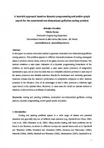
The second situation is illustrated in Fig. 3 as Scenario III. In this scenario, transportation costs are involved to execute Query Q1 . Then, we get:
f1
f1
a4
f1+f2
f1 a2
a3
costsλ2 ≈ transλ1 (Q1 ) = f1 · (`1 + `2 + `3 + `4 ) · c21 Assuming f2 > f1 , if we do not perform vertical fragmentation using affinities but consider both vertical fragmentation and allocation together to find an optimal solution we can have two fragments Fu1 = {a1 , a2 } Fu2 = {a3 , a4 } and allocate Fu2 to site N2 . This fragmentation and allocation are illustrated in Scenario IV in Fig. 4. In this case, total query costs are costλ3 ≈ transλ2 (Q1 ) = f1 · (`3 + `4 ) · c21 Assuming c12 = c21 = 1, we compare query costs in Scenario IV to that in Scenario II and get costλ1
= costλ3 + f2 · (`3 + `4 ) − f1 · (`3 + `4 ) = costλ3 + (`3 + `4 ) · (f2 − f1 ) >
costλ3
Fu a1
f1
f1 a2
Fig. 1.
f1
a4
f1+f2 a3
Scenario I: Fragmentation with two queries at one location
=f1 *(l1 +l2 +l3 +l4)
Fig. 3.
Scenario III: Fragmentation with two queries at different location
Comparing with query costs in Scenario IV to that in Scenario III, we get costλ2
= costλ3 + f1 · (`1 + `2 + `3 + `4 ) − f1 · (`3 + `4 ) = costλ3 + f1 · (`1 + `2 )
> costλ3 Obviously, the fragmentation and allocation in Scenario IV is the best solution, which results from comparing with query costs while making decision of fragmentation. That is, to get an optimal solution of fragmentation and allocation we need to employ a cost model, with which we can achieve an optimal fragmentation and allocation simultaneously. With the cost model, any change of the query information, including the site information of queries, will be reflected in the design of fragmentation and allocation. But the approaches of vertical fragmentation using the value of affinities can not reflect this change. However, if a relation has m nonprimary key attributes, the possible fragments are given by the Bell number which is approximately B(m) ≈ mm . With this number of possible fragments, the following up allocation, using the cost model m introduced previously, is of the complexity k (m ) with k as the number of network nodes. Therefore, it is impossible to get the
Fu1
f1
a1
Fu2
a4
f1+f2
f1 a2
a3
ff11
=f1 *(l3 +l4)
Fig. 4.
Scenario IV: Fragmentation with two queries at different location
optimal solutions to the vertical fragmentation and allocation problems. We can only expect to find a heuristic solution. In the remaining of this section, we first define some terms. Then we introduce a heuristic approach to vertical fragmentation and allocation. This approach adapts a simplified cost model while making decision of vertical fragmentation.
other indicating the frequency of the queries. The values on a column indicate the frequency fji of the query Qj that use the corresponding attributes ai grouped by the site that issues queries. Note that we treat the same query at different sites as different queries. Doing this way we only need one matrix to record all the information rather than two matrices, Attribute Usage Matrix and Access Matrix, that are used in [9]. Subsequently, the following up calculation is easy to be formulated. From one site each attribute is requested by multiple queries. The request of an attribute at a site h is the sum of frequencies of all queries at the site accessing the attribute. It can be calculated with the formula below: m X fji requesth (ai ) = j=1,λ(Qj )=h
Let fji be the frequency of a query accessing to an attribute ai of a fragment Fu of a type E, li be the length of the attribute. The need of a fragment at a site h is calculated with the following formula: needh (Fu ) =
n X
`i · fji
j=1,λ(Qj )=h i=1,ai ∈Au
B. Requests and Needs at Sites We now define some terms that will be used in our discussion. Assume a relation R = {a1 , . . . , an } being accessed by a set of queries Qm = {Q1 , . . . , Qj , . . . Qm } with frequencies f1 , . . . , fm , respectively. To improve the system performance, relation R is vertically fragmented into a set of fragments {F1 , . . . , Fu , . . . , Fv }, each of which is allocated to one of the network nodes N1 , . . . , Nh , . . . , Nk . Each attribute ai of R is of average length `i . Note that the maximum number of fragments is k, i.e.,v ≤ k. We use λ(Qj ) to indicate the site that issues query Qj , and use Aj = {ai |fji = fj } to indicate the set of attributes that are accessed by Qj , with fji as the frequency of the query Qj accessing attributes ai . Here, fji = fj if the attribute ai is accessed by Qj . Otherwise, fji = 0. From the discussion in the previous section we know that to get a optimal vertical fragmentation we need to employ a cost model which take input information as: • the frequency of queries that access the object; when the same query is issued at different sites, it is treated as different queries; • the subset of the attributes used by queries; • the size of each attribute of the object. • the site that issue the queries To record the above input information we introduce Attribute Usage Frequency Matrix (AUFM). Each row represents one query Qj ; the head of column is the set of attributes of a relation E. In addition, there are two columns with one column indicating the site that issues the queries and the
m X
or needh (Fu ) =
m X
sji · fj
j=1,λ(Qj )=h
with sji as the size of data volume required by query Qj from fragment Fu . We can also calculate the need of an attribute using the above formula.
needh (ai )
= `i ·
m X
fji
j=1,λ(Qj )=h
= `i · request(ai ) In distributed databases, costs of queries are dominated by the cost of data transportation from a remote site to the site that issued the queries. To compare different vertical fragmentation schemata we would like to compare how it affect the transportation costs. So we can simplify the cost model in Section II-B as following: costλ =
m X v X
needh (Fu ) · chh0
(?)
h=1 u=1
Note that the cost factor chh0 = 0, if h = h0 . Example 3: Assume a fragment F being accessed by three queries from three different sites, a, b, c, respectively. If we allocate fragment F to site c, λ(F ) = c, then the costs of all queries that access this attribute can be calculated by summing up the need at site a multiply with the cost factor cca and the
need at site b multiply with the cost factor ccb . Using formula (?) we have: costλ(F )=c = needa (F ) · cca + needb (F ) · ccb Finally, we introduce a term pay to measure the costs of allocating a single attribute to a network node. The pay of allocating an attribute ai to a site h measures the costs of accessing attribute ai from all queries at the other sites h0 , which is different from h. It can be calculated using the following formula: k X
payh (ai ) =
requesth0 (ai ) · chh0
h0 =1,h6=h0
We do not include attribute length in the formula because when we compare the pay of an attribute at different sites, attribute length will always be the same. C. Heuristics for Vertical Fragmentation As in [8], we assume a simple transaction model, using which the system collects the information at the site of the query and executes the query there. In this case we can evaluate costs of allocating a single attribute to network nodes and then make decision by choosing a site that leads to the least query costs. Also, according to our discussion of how vertical fragmentation affect query costs, the allocation of fragments to network nodes, following the cost minimisation heuristics, already determine the location assignment provided that an optimal location assignment for the queries was given prior to the fragmentation. Taking the simplified cost model introduced above we now analyse the relationships between cost, the pay and the request. We compute the following fomulae: costh (ai ) =
k X
needh0 (ai ) · chh0
h0 =1,h6=h0
=
m X
k X
`i · fji · chh0
h0 =1,h0 6=h j=1,λ(Qj )=h0
= `i ·
k X
h0 =1,h0 6=h
= `i ·
k X
m X
j=1,λ(Qj
fji · chh0 )=h0
requesth0 (ai ) · chh0
h0 =1,h0 6=h
= `i · payh (ai ) The above formula gives rise to two alternative heuristics for the allocation of an attribute ai (i = 1, . . . , n). • The first heuristic allocates ai to a network node Nw such that payw (ai ) is minimal, i.e., we choose a network node in such a way that the total transport costs for all queries arising from the allocation are minimised.
The second heuristic allocates ai to a network node Nw such that requestw (ai ) is maximal. i.e., we choose the network node with the highest request of the attribute ai . This guarantees that there are no transport costs associated with data of attribute ai for those queries that need the data of ai most frequently. In addition, the availability of data of attribute ai will be maximised. Taking the first heuristic we perform vertical fragmentation with the following steps. We do not distinguish read and write queries because replication is not considered at this stage. The second heuristic is easy to be formulated. 1) Take the most frequently used 20% queries QN . 2) Optimise all the queries and construct an AUFM for each database type R based on the queries. 3) Calculate the request at each site for each attribute to construct an Attribute request Matrix. 4) Calculate the pay at each site for each attribute to construct an Attribute pay Matrix. 5) Cluster all attributes to the site which has the lowest value of the pay. 6) Attach the primary key to each of the fragments. This procedure is formally described as the algorithm below. Algorithm 1 (Allocation of Vertical Fragments): Input: QN = {Q1 , . . . , Qn } /* a set of queries R = {a1 , . . . , an } /* a type with a set of attributes a set of network nodes N = {1, . . . , k} The AUFM of R Output: vertical fragmentation schema and fragment allocation schema Begin for each h ∈ {1, . . . , k} let Fh = ∅ endfor for each attribute ai ∈ R, 1 ≤ i ≤ n do for each node h ∈ {1, . . . , k} do calculate requesth (ai ) endfor for each node h ∈ {1, . . . , k} do calculate payh (ai ) endfor choose w such that payw (ai ) = minkh=1 payh (ai ) /* find the minimum add ai to Fw /* allocate the attribute into the corresponding node endfor The above algorithm first finds the site that has the smallest value of the pay then allocates the attribute to the site. A vertical fragmentation and allocation schema are obtained simultaneously. •
D. Discussion The advantages of our heuristic approach for vertical fragmentation and fragment allocation are:
•
•
•
•
Except key attributes, there is no overlap among all the vertical fragments. Therefore, we do not need extra procedure to remove overlaps. The change of queries will be reflected by the fragmentation solution. Query information may reflect the needs to retain attributes from some sites more often than some other sites. Even though on the affinity graph the cutting edges will be the same. The complexity of this approach is low. Lets m be the number of queries, n be the number of attributes, k be the number of network nodes. The complexity of our approach, which dealing with vertical fragmentation and allocation, is O(m · n + k 2 · n), while the complexity of graphical approach in [9] is O(n2 · m + k n ) for the whole design procedure, including building the affinity matrix, vertical fragmentation and allocation. This approach suits the situation that for each relation the number of attributes is small and the number of queries is big. Usually, the number of queries taken into consideration is bigger than the number of attributes of a relation.
E. An Example We will take the same example problem in [8], [9] to illustrate how our approach works and compare our fragmentation decision with that in [8], [9]. Firstly, we take the Attribute Usage Matrix and Attribute Access Matrix in [8] to construct an AUFM grouped by site that issues the queries. The AUFM is shown in Table I. Secondly, we compute the request for each attribute at each site and get the a Attribute request Matrix shown in Table II. Thirdly, assuming we have been given the values of transportation cost factors in Table III, we can now calculate the pay of each attribute at each site using the values of the request in Table II and values of cost factors in Table III. The results are shown in a Attribute pay Matrix in Table IV. Finally, for each attribute we compare all the pay at all sites to find the minimal one. We then allocate attribute ai to the site that of the minimal pay. The allocation of attribute is shown in Table V. Therefore, relation R has been fragmented into two fragments with F1 = {a1 , a2 , a3 , a5 , a7 , a8 , a9 } and F2 = {a4 , a6 , a10 }, which have been allocated to site 2 and 3 respectively. TABLE III T RANSPORTATION C OST FACTORS site 1 2 3 4
1 0 10 25 20
2 10 0 20 15
3 25 20 0 15
4 20 15 15 0
TABLE V ATTRIBUTE ALLOCATION
attribute ai site Nj
1 2
2 2
3 2
4 3
5 2
6 3
7 2
8 2
9 2
10 3
Lets now compare our fragmentation schema with the fragmentation decision in [8], [9]. In [8], [9] the relation is first fragmented into three fragments: F1 = {a1 , a5 , a7 }, F2 = {a2 , a3 , a8 , a9 } and F3 = {a4 , a6 , a10 }. Then, at the refinement stage, F1 and F2 are allocated at the same site. That means that the final fragmentation schema is {a1 , a2 , a3 , a5 , a7 , a8 , a9 }, {a4 , a6 , a10 }, which is same as our results. However, our approach is of less complexity. Lets take the example problem in [8] again and move all queries T2 from site 2 to site 1. In this case, the affinity graph does not change; therefore the resulting fragmentation schema is not changed. But using our approach we get a different fragmentation schema, {a2 , a8 }, {a1 , a3 , a5 , a7 }, {a4 , a6 , a10 }. To compare the two solutions we use the simplified cost model introduced in Section III. The total query costs result from fragmentation schema {a2 , a8 }, {a1 , a3 , a5 , a7 }, {a4 , a6 , a10 } is 64255 and the optimal allocation of fragmentation schema {a1 , a5 , a7 }, {a2 , a3 , a8 , a9 }, {a4 , a6 , a10 } is 64580. Obviously, our approach leads to a better design because the change of input query information is reflected in the decision of fragmentation to reduce the total query costs. We conclude that our heuristic approach to vertical fragmentation improves the deficiencies of all the other vertical fragmentation approaches, which make decision according to the affinities between each pair of attributes, by introducing a simplified cost model at the stage of vertical fragmentation. Also, the vertical fragmentation algorithm is of lower complexity than the vertical fragmentation algorithms using affinities. IV. C ONCLUSION In this paper we presented a heuristic approach to vertical fragmentation for relational datamodel. The major objective is to provide a tractable approach to minimising the query processing costs for the most frequent queries. In general, this would require to consider all possible fragmentations and all possible allocations of intermediate query results to the nodes of a network, which is intractable. Instead of this we suggest to consider vertical fragmentation and allocation using cost model at the same time. The next step of our work is to adapt the heuristic approach to complex value databases, which cover the common aspects of object-oriented databases, object-relational databases, and databases based on the eXtensible Markup Language (XML). For this, complex data types should be covered by the cost model. The procedure of vertical fragmentation should be altered accordingly. Also, we need to integrate the handing
TABLE I ATTRIBUTE U SAGE F REQUENCY M ATRIX Site 1 1 1 1 1 1 1 2 2 2 2 2 2 3 3 3 3 3 3 3 4 4 4 4 4 4 4 Length
Query T1 T2 T4 T6 T5 T7 T8 T2 T1 T5 T7 T6 T8 T3 T4 T2 T5 T6 T7 T8 T2 T3 T4 T5 T6 T7 T8
Frequency 10 10 10 10 5 5 5 20 15 10 10 5 5 15 15 10 5 5 5 3 10 10 10 5 5 5 2
a1 10 0 0 10 5 0 0 0 15 10 0 5 0 0 0 0 5 5 0 0 0 0 0 5 5 0 0 10
a2 0 10 10 0 5 0 0 20 0 10 0 0 0 0 15 10 5 0 0 0 10 0 10 5 0 0 0 8
a3 0 10 0 0 5 5 5 20 0 10 10 0 5 0 0 10 5 0 5 3 10 0 0 5 0 5 2 4
a4 0 0 0 0 0 0 5 0 0 0 0 0 5 15 0 0 0 0 0 3 0 10 0 0 0 0 2 6
a5 10 0 0 10 5 0 0 0 15 10 0 5 0 0 0 0 5 5 0 0 0 0 0 5 5 0 0 15
a6 0 0 0 0 0 0 5 0 0 0 0 0 5 15 0 0 0 0 0 3 0 10 0 0 0 0 2 14
a7 10 0 10 0 5 0 0 0 15 10 0 0 0 0 15 0 5 0 0 0 0 0 10 5 0 0 0 3
a8 0 10 10 0 5 0 0 20 0 10 0 0 0 0 15 10 5 0 0 0 10 0 10 5 0 0 0 5
a9 0 10 0 0 5 5 5 20 0 10 10 0 5 0 0 10 5 0 5 3 10 0 0 5 0 5 2 9
a10 0 0 0 0 0 0 5 0 0 0 0 0 5 15 0 0 0 0 0 3 0 10 0 0 0 0 2 12
TABLE II ATTRIBUTE request M ATRIX Site 1 2 3 4
Query request request request request
Frequency
a1 25 30 10 10
a2 25 30 30 25
a3 25 45 23 22
a4 5 5 18 12
a5 25 30 10 10
a6 5 5 18 12
a7 25 25 20 15
a8 25 30 30 25
a9 25 45 23 22
a10 5 5 18 12
9 1465 1040 1855 1520
10 740 590 405 445
TABLE IV ATTRIBUTE pay M ATRIX attribute pay1 (ai ) pay2 (ai ) pay3 (ai ) pat4 (ai )
1 750 600 1375 1100
2 1550 1225 1600 1400
3 1465 1040 1855 1520
4 740 590 405 445
of horizontal fragmentation, which has been discussed in [6], and vertical fragmentation with the consideration of the requirement of global optimisation. R EFERENCES [1] P. M. G. Apers, “Data allocation in distributed database systems,” ACM Transactions on Database Systems, vol. 13, pp. 263–304, 1988. [2] S. Chakravarthy, J. Muthuraj, R. Varadarajan, and S. Navathe, “An objective function for vertically partitioning relations in distributed databases and its analysis,” University of Florida, Gainesville, FL, Tech. Rep. UF-CIS-TR-92-045, 1992.
5 750 600 1375 1100
6 740 590 405 445
7 1050 875 1350 1175
8 1550 1225 1600 1400
[3] D. Cornell and P. Yu, “A vertical partitioning algorithm for relational databases,” in International Conference on Data Engineering, Los Angeles, California, 1987, pp. 30–35. [4] H. Ma, “Distribution design in object oriented databases,” Master’s thesis, Massey University, 2003. [5] H. Ma, K.-D. Schewe, and Q. Wang, “Distribution design for higherorder data models,” Massey University, Tech. Rep. 11/2005, 2005. [6] ——, “A heuristic approach to cost-efficient fragmentation and allocation of complex value databases,” in Proc. ADC 2006, ser. CRPIT, G. D. J. Bailey, Ed., vol. 49, Hobart, Australia, 2006. [7] J. Muthuraj, S. Chakravarthy, R. Varadarajan, and S. B. Navathe, “A formal approach to the vertical partitioning problem in distributed database design,” in Proc. The Second International Conference on Parallel and
Distributed Information Systems, San Diego, CA, USA, Jan 1993. [8] S. B. Navathe, S. Ceri, G. Wiederhold, and J. Dour, “Vertical partitioning algorithms for database design,” ACM TODS, vol. 9, no. 4, pp. 680–710, 1984. [9] S. B. Navathe and M. Ra, “Vertical partitioning for database design: A graphical algorithm,” SIGMOD Record, vol. 14, no. 4, pp. 440–450, 1989. ¨ [10] M. T. Ozsu and P. Valduriez, Principles of Distributed Database Systems. New Jersey: Alan Apt, 1999.