A Heuristic for Generating Scenario Trees for Multistage Decision Problems. Kjetil Høyland â. Michal Kaut â . Stein W. Wallace â¡. June 20, 2000; revised April 6, ...
A Heuristic for Generating Scenario Trees for Multistage Decision Problems Kjetil Høyland
∗
Michal Kaut
†
Stein W. Wallace
‡
June 20, 2000; revised April 6, 2001
Abstract In stochastic programming models we always face the problem of how to represent the uncertainty. When dealing with multidimensional distributions, the problem of generating scenarios can itself be difficult. We present an algorithm for efficient generation of scenario trees for single or multi-stage problems. The presented algorithm generates a discrete distribution specified by the first four marginal moments and correlations. The scenario tree is constructed by decomposing the multivariate problem into univariate ones, and using an iterative procedure that combines simulation, Cholesky decomposition and various transformations to achieve the correct correlations. Our testing shows that the new algorithm is substantially faster than a benchmark algorithm. The speed-up increases with the size of the tree and is more than 100 in a case of 20 random variables and 1000 scenarios. This allows us to increase the number of random variables and still have a reasonable computing time. Keywords: stochastic programming, scenario tree generation, asset allocation, Cholesky decomposition, heuristics
1
Introduction
Gjensidige Nor Asset Management (GNAM) has NOK 65 billion (7 billion US$) under management. During the last few years they have used stochastic-programming-based asset allocation models in their asset allocation processes. The most important step in that process is to establish the market expectations, i.e. to establish what are their beliefs for the major asset categories (bonds, stocks, cash, commodities and currencies) in different major regions of the world. The decision-makers prefer to express their expectations in terms of marginal distributions of the return / interest rates for the different asset classes in addition to correlations. The challenge in converting these expectations into an asset allocation mix is twofold: First we need to convert the expectations into a format which a stochastic programming model can handle, second we need an optimisation model which gives us the optimal asset mix, given this input. Practical experience has told us that the first part, the scenario generation, can in fact be the most challenging and (computer-) time consuming one. For the purpose of generating the input data, GNAM has been using the method described in Høyland and Wallace, 2001, a method developed in 1996. For larger problems with many asset classes the scenario generation became the bottleneck in the portfolio optimisation process. This paper presents an algorithm that reduces the computing time for the scenario generation substantially. The most well-known applications of asset allocation models are the Russell Yasuda Kasai model in Cari˜ no and Ziemba, 1998 and the models implemented by Towers Perrin in Mulvey, 1996. Other applications can be found in Consigli and Dempster, 1998 and Dert, 1995. These models are all focused on long term strategic asset liability planning. Stochastic processes are widely used for scenario generation in such models. The big challenge with such ∗
Gjensidige Nor Asset Management, POBox 276, N-1326 Lysaker, Norway Dept. of Industrial Economics and Technology Management, NTNU, N-7491 Trondheim, Norway ‡ Centre for Advanced Study, Norwegian Academy of Science and Letters, N-0271 Oslo, Norway †
1
processes is to calibrate the parameters so that the generated scenarios are consistent with the decision-maker’s beliefs of the future development of the asset classes. In many applications the parameters are calibrated so that the future scenarios are consistent with the past. This might be acceptable for long term strategic planning. For tactical short term planning, i.e. for the question of how to construct an asset allocation mix relative to an asset allocation benchmark, such approaches are, however, inappropriate. The user wishes to express views on the future which deviate from the past. It is then important that the decision-maker can express the market expectations in a way that he or she finds convenient and that these expectations are converted to model input in a consistent manner. This is the basic philosophy of the scenario generation method proposed in Høyland and Wallace, 2001. The user specifies his or her market expectations in terms of marginal distributions for each asset class in addition to correlations between the different asset classes and possibly other statistical properties. The stochastic, possibly multi-period, asset allocation model requires discrete outcomes for the uncertain variables. To generate these outcomes a regression model is applied. The idea is to minimise the distance between the statistical properties of the generated outcomes and the specified statistical properties (specified either directly or derived from the marginal distributions), see Høyland and Wallace, 2001 for more details. In the general form of the algorithm presented in Høyland and Wallace, 2001 all the random variables (returns for all the asset classes) are generated simultaneously. Such an approach becomes slow when the number of random variables increases. In this paper we present an algorithm that decomposes the scenario generation problem. We generate one marginal distribution at a time and create the multivariate distribution by putting the univariate outcomes ‘on top of each other’, i.e. by creating the i-th multivariate outcome as a vector of the i-th outcomes of all the univariate distributions. We then apply various transformations in an iterative loop to reach the target moments and correlations. The presented algorithm is inspired by the work of Fleishman, 1978, Vale, 1983 and Lurie and Goldberg, 1998. Fleishman presents a cubic transformation that transforms a sample from a univariate normal distribution to a distribution satisfying some specified values for the first four moments. Vale and Maurelli address the multivariate case and analyse how the correlations are changed when the cubic transformation is applied. The algorithm assumes that we start out with multivariate normals. The initial correlations are adjusted so that the correlations after the cubic transformation are the desired ones. The algorithm is only approximate with no guarantee about the level of the error. Lurie and Goldberg outlined an algorithm that is of similar type as ours. They also generate marginals independently and transform them in an iterative procedure. There are, however, two major differences between the two algorithms. One is in the way they handle the (inevitable) change of distribution during the transition to the multivariate distribution – while they modify the correlation matrix in order to end up with the right distribution, we modify the starting moments. The other major difference is that they start out with parametric univariate distributions whereas we start out with the marginal moments. We believe that specifying marginal moments is a more flexible approach and we certainly could also derive the marginal moments (up to the desired number) from the parametric distribution and apply our approach. In Section 2 we present the algorithm. To simplify the presentation the algorithm is illustrated for the single period case. Høyland and Wallace argue that the quality1 of the scenario tree improves if several small trees are aggregated to a larger tree rather than generating the larger tree directly. We present the algorithm for a single period with no aggregation. In Section 3 we discuss how the algorithm can be adjusted to incorporate tree aggregation and multiple periods. Numerical results are presented in Section 4, while possible future research areas are discussed in Section 5.
2
The algorithm
In Høyland and Wallace’s method a scenario tree can in principle be constructed to fit any statistical properties. In this section we will assume that the specified properties are the first four marginal moments and the correlations. This is consistent with many other studies, as 1
See Høyland and Wallace, 2001 for how to measure ‘quality’ of the scenario tree.
2
well as our own empirical analyses in Høyland and Wallace, 2001 of what were the important statistical properties. The presented methodology is more general than this, we could in principle specify even higher moments, but it is more restrictive than our original approach, where a wide range of statistical properties could be specified. The general idea of the algorithm is as follows: Generate univariate outcomes for n random variables each satisfying a specification for the first four moments. Transform these outcomes so that the new outcomes are consistent with a correlation matrix. The transformation will distort the higher than the second moments of the original univariate outcomes. Hence we need to start out with a different set of higher moments so that the higher moments that we end up with are the right ones. The procedure would lead to the exact desired values for the correlations and the marginal moments if the generated univariate outcomes were independent. This is, however, true only when the number of scenarios goes to infinity. With a limited number of scenarios, the marginal moments and the correlations will therefore not fully match the specifications. To be able to secure that the error is within a pre-specified range we have developed an iterative algorithm, which is an extension of the core algorithm. Section 2.1 discusses the assumptions we have on the correlation matrix, Section 2.2 introduces necessary notation, Section 2.3 explains the key transformations used in the algorithm, Section 2.4 describes the core module of the algorithm, while Section 2.5 explains the iterative procedure.
2.1
Assumption on the correlation matrix
There are two assumption on the specified correlation matrix R. The first one is a general assumption that R is a possible correlation matrix, i.e. that it is a symmetric positive semidefinite matrix with 1’s on the diagonal. While implementing the algorithm there is no need to write a special code that controls the positive semi-definiteness, because we do a Cholesky decomposition of the matrix R at the very start. If R is not positive semi-definite, the Cholesky decomposition will fail. Note that having an R that is not positive semi-definite means having some internal inconsistency in the data, so we should re-run our analysis. As an alternative, there exist several algorithms that find a possible correlation matrix that is, in some sense, closest to the specified matrix R. One such an algorithm can be find in Higham, 2000. Another approach is used in Lurie and Goldberg, 1998, where a QP model is formulated to solve the problem. The latter approach has an advantage of being very flexible and allowing, for example, for specifying weights that express how much we believe in every single correlation. We can also used bounds to restrict the possible values. On the other hand, it has the obvious disadvantage of needing a QP solver. The other assumption is that all the random variables are linearly independent, so R is nonsingular – hence positive definite – matrix. For checking this property we can use again the Cholesky decomposition, because the resulting lower-triangular matrix L will have zero(s) on its diagonal in a case of linear dependency. This is not a serious restriction, since having a linearly dependent variable mean that it can be computed from the others after the generation, and we can thus decrease the size of the problem. If we are not sure about our correlations, we can use the method from Lurie and Goldberg, 1998 mentioned in the previous paragraph to enforce the positive definiteness. Since they have the elements of the Cholesky-decomposition-matrix Lij as variables in the QP model, we can simply add a constraint {Lii ≥ ε > 0} for every random variable i. We also suggest a simple heuristic to handle the singularity of the correlation matrix inside our algorithm, see Section 2.5.1 It is, however, a very crude procedure, and we recommend to avoid singular correlation matrices if possible by going back to the analysis of the data.
2.2
Notation
To formulate the model we introduce the following notation. Note that vectors are columns by default. n s ˜ X
number of random variables number of scenarios n-dimensional random variable
3
X X Xi ˜ X(mom; corr)
˜ i is an ith marginal of X ˜ → X ˜ → every moment of X is a vector of size n ˜ is a matrix of size n × n → correlation matrix of X ˜ – vector of size n one realisation of random variable X ˜ – X has dimension n × s matrix of s outcomes of random variable X ˜ i – Xi has size s row vector of outcomes for random variable X ˜ X has moments mom = mom1 . . . mom4 and a correlation matrix corr – every momi is a vector of size n, and corr is a matrix of size n × n
Our goal is to generate outcomes Z from an n-dimensional random variable Z˜ with properties ˜ Z(T ARM OM ; R), i.e. T ARM OM is the matrix (of size 4 × n) of target moments and R is the target correlation matrix (of size n × n).
2.3
Key transformations
The core module, which will be presented in the next section, has two key transformations. One is a cubic transformation used for generating univariate distributions with specified moments. The other is a matrix transformation used to transform the multivariate distribution to obtain a given correlation matrix.
2.3.1
Cubic transformation
This transformation comes from Fleishman, 1978, where a method to simulate an univariate non-normal random variable Y˜i with given first four moments is introduced.2 It takes a N (0, 1) ˜ i and uses a cubic transformation variable X ˜ i + cX ˜ i2 + dX ˜ i3 Y˜i = a + bX to obtain Y˜i with the target moments. Parameters a, b, c and d are found by solving a system of ˜i. non-linear equations. Those equations utilise normality of the variable X ˜ i must have the first 12 moments equal to those of The problem of this approach is that X N (0, 1) in order to get exactly the target moments of Y˜i . Since this is hard to achieve, either by sampling or discretisation, the results with those formulas are only approximate. We have thus dropped the assumption of normality and derived formulas that work with arbitrary random ˜ i – see Appendix C. Parameters a, b, c and d are now given by a system of four implicit variable X equations. We have used a simple mathematical-programming (regression) model to solve the system. In this model we have a, b, c and d as independent variables, moments of Y˜i as dependent variables, and we minimise a distance of the moments from their target values. Other possibilities for solving the system are for example using Matlab routines or some variant of Newton’s method. Note that unlike the normal case,3 the parameters depend not only on the target moments ˜ ˜ i . Our method for generating a sample Yi from Y˜i is of Yi , but also on the first 12 moments of X then following: • • • •
take some sample Xi of the same size as Yi calculate the first 12 moments of Xi (as a discrete distribution) compute the parameters a, b, c, d construct Yi as Yi = a + bXi + cX2i + dX3i
2.3.2
Matrix transformation
Our other main tool in the algorithm is a matrix transformation ˜ Y˜ = L × X 2 3
The index i is obsolete in this section, but we use it for consistence with the rest of the paper. ˜ i also when X ˜ i is normal, but we know their values in advance. Parameters depend on the first 12 moments of X
4
where L is the lower-triangular matrix. The matrix L always comes from a Cholesky decomposition of the correlation matrix R, so we have L × LT = R.4 ˜ is an n-dimensional N (0, 1) random variable From the statistical theory we know that if X ˜ i mutually independent), then the Y˜ = L × X ˜ is with correlation matrix I (and therefore with X an n-dimensional N (0, 1) random variable with correlation matrix R = L × LT . Since we do not have normal variables, we need a more general result. To make the formulas as simple as possible, we restrict ourselves to the case of zero means and variances equal to 1. ˜ =0 In the beginning of Section 2.4 we show how to deal with this restriction. Note that E[X] ˜ i ]. We will thus use the two interchangeably for the rest of the section. leads to momi = E[X ˜ i have zero mean, variance equal to 1, and are mutually In Appendix B we show that if the X ˜ is an n-dimensional independent, and if R = L × LT is a correlation matrix, then Y˜ = L × X random variable with zero means, variances equal to 1, and correlation matrix (which is also the variance-covariance matrix) R. Its marginals Y˜i have higher moments: i X � � � � E Y3i = L3ij E X3j j=1
� � E Y4i − 3
=
i X
� � � L4ij E X4j − 3
j=1
We will need also the opposite direction of the transformation: ˜ = L−1 × Y˜ X ˜ can Since the above formulas are triangular, it is easy to invert them. The higher moments of X be then express as: i−1 X � 3� � � � � 1 E Xi = E Y3i − L3ij E X3j L3ii j=1 i−1 X � 4� � � � � � 1 E Xi − 3 = E Y4i − 3 − L4ij E X4j − 3 L4ii j=1 We divide only by the diagonal elements Lii in these formulas. We can do it since Lii are positive due to regularity (positive definiteness) of R. Note however that if Lii are close to zero, we can experience numerical problems. See remark at the end of Appendix B for how to check for this problem in advance, or Section 2.5.1 for how to deal with it inside the algorithm. Having both directions of the transformation allows us to transform random variables from one correlation matrix to another. First we transform the variables so that they are independent using the inverse formulas and then we use the original formulas to transform variables to the target correlation matrix. We will use that later in the algorithm.
2.4
The core algorithm
This section presents the core algorithm. It runs as follows: Find the target marginal moments. Generate n univariate discrete distributions that satisfy those moments. Create a multivariate distribution by putting the univariate outcomes ‘on top of each other’ in the order they coincidentally were generated. (We can do this since all the univariate distributions have the same size and the same fixed probabilities for the corresponding outcomes.) Transform these outcomes so that they have the desired correlations and marginal moments. If the discrete distributions Xi were independent, we would end up with a sample having exactly the desired properties. For an easier orientation in the algorithm, we have divided it in two parts. In the input phase we read the target properties specified by the user and transform them to a form needed by the algorithm. In the output phase we generate the outcomes and transform them to the original properties. 4
Note that L always exists, since we assume R to be positive semi-definite.
5
2.4.1
The input phase
In this phase we work only with the target moments and correlations, we do not have any outcomes yet. This mean that all the operations are fast and independent on the number of scenarios s. Our goal is to generate an n-dimensional random variable Z˜ with moments T ARM OM and a correlation matrix R. Since the matrix transformation needs zero mean and variance equal to 1, we have to change the targets to match this demand. Instead of Z˜ we will thus generate random variables Y˜ with properties Y˜ (M OM ; R), M OM1 = 0, and M OM2 = 1. Z˜ is then computed at the very end of the algorithm as Z˜ = αY˜ + β In Appendix A we show that the values leading to the correct Z˜ are: T ARM OM3 α3 T ARM OM4 M OM4 = α4
1/
M OM3 =
α = T ARM OM2 2 β = T ARM OM1
The final step in the input phase is to derive moments of independent 1-dimensional variables ˜ i such that Y˜ = L × X ˜ will have the target moments and correlations. To do this we need to X find the Cholesky-decomposition matrix L, i.e. a lower-triangular matrix L so that R = L × LT . The input phase then contains the following steps: 2.
Specify the target moments T ARM OM and target correlation matrix R of Z˜ Find the ‘normalised moments M OM of Y˜
3.
˜ — see Section 2.3.2 Compute L and find the transformed moments T RSF M OM of X
1.
user
~
Step 1
Step 2
Z
TARMOM, R
~
Y
MOM, R
Step 3
~
X
TRSFMOM, I
Figure 1: Input Phase
2.4.2
The output phase
In this phase we generate the independent outcomes, transform them to get the intermediatetarget moments and the target correlations and finally transform them to the moments specified by the user. Since the last transformation is a linear one, it will not change the correlations. All the transformations in this phase are with the outcomes, so the computing time needed for this phase is longer and increases with the number of scenarios s. ˜ i independently, one We start by generating discretisations of the univariate distributions X by one. This is a well-known problem and there are several possible ways to do it. We have used a method from Fleishman, 1978, in a way described in Section 2.3.1. The method starts by sampling from N (0, 1) and afterwards uses the cubic transformation to get the desired moments. For the starting N (0, 1) sample we use a random-number generator. An alternative would be to use a discretisation based on the distribution, or some other method for the starting N (0, 1) sample. Another possibility is to use the method described in Høyland and Wallace, 2001. They ˜ i as independent variables and the formulate a non-linear regression model with outcomes of X first four moments as dependent variables. The distance (sum of squares) of the actual moments from the target moments is then minimised.
6
˜ i , we can proceed with the transOnce we have generated the outcomes Xi of marginals X formations. First Y = L × X to get the target correlations and then Z = αY + β to get the user-specified moments5 . The output phase of the core algorithm consists of the following steps: ˜ i (independently for i = 1 . . . n) 4. Generate outcomes Xi of 1-dimensional variables X 5. Transform X to target correlations: Y = L × X → Y is Y˜ (M OM ; R) 6.
˜ ARM OM ; R) Transform to original moments: Z = αY + β → Z is Z(T
Step 4
X
Step 5
Step 6
Y
TRSFMOM, I
MOM, R
Z
user
TARMOM, R
Figure 2: Output Phase
2.5
The modified algorithm
We know that the core algorithm gives us the exact results only if the random variables having support Xi are independent. Since we generate each set of outcomes Xi separately and have a limited number of outcomes (s), the sample co-moments will most certainly differ from zero and the results of the core algorithm will be only approximate. The modified algorithm is iterative, so all results are approximate, with a pre-specified max˜ this time both forward imal error. We will again use the matrix transformation Y˜ = L × X, and backward, as mentioned in 2.3.2. Recall that this transform allows us to obtain a desired correlation matrix, but it changes the moments while doing it. In Section 2.3.1 we showed that the cubic transformation allows us to transform the general ˜ to a variable with some target moments. This transformation univariate random variable X ˜ is close to the target distributions, the change in changes the correlations, but if the starting X the correlations is expected to be small. Our idea is thus to apply the cubic and the matrix transformation, alternately, hoping that the algorithm converges and outcomes with both right moments and correlations are achieved. This introduces the iterative loops to the core algorithm, namely to Steps 4 and 5, in the following way: In Step 4 we would like to generate the independent outcomes Xi . Since independence is very hard to achieve, we change our target to generating uncorrelated outcomes Xi , i.e. we seek to get ˜ RSF M OM ; I). We use an iterative approach to achieve those properties. X with properties X(T Since we do not control the higher co-moments, they will most likely not be zero, and the Y obtained in Step 5 will not match the target properties. We thus need another loop there to end up with the desired Y. The iterative versions of Steps 4 and 5 are6 : Step 4 4.i. 4.ii. 4.iii. 4.iv. 4.v.
Generate n marginals with target moments T RSF M OM (independently) → we get X with correlation matrix R1 close to I due to independent generation let p = 1 and X1 = X while dist(Rp ; I) > εx do do Cholesky transformation: Rp = Lp × LTp do backward transform X∗p = L−1 × Xp → zero correlations, wrong moments
5 Note that we have stopped to speak about distributions and started to speak about outcomes, so we have to ˜ to X change the notation from X 6 As we have not found any better notation, in the rest of this section lower index p denotes an iteration counter, not a matrix column.
7
4.vi. 4.vii. 4.viii. 4.ix.
do cubic transform of X∗p with T RSF M OM as the target moments; store results as Xp+1 → right moments, wrong corr. compute correlation matrix Rp+1 let p = p + 1 ˜ RSF M OM ; I) with correlation error dist(Rp ; I) ≤ εx let X = Xp → X is from X(T
The sum of squares of differences of elements is used as a distance of two matrices in 4.iii. The same distance is used also at points 5.iii and 5.ix below. Since X is not a final output, the maximum error εx in Step 4 is typically higher than the corresponding εy in Step 5. There are two possible outcomes from Step 4: Xp corresponding to random variables with ∗ right moments and wrong correlations, and Xp−1 corresponding to random variables with slightly off moments and zero correlations. We start with the latter in the Step 5, and denote it X ∗ . Step 5 5.i. 5.ii. 5.iii. 5.iv. 5.v. 5.vi. 5.vii. 5.viii. 5.ix.
Y1 = L × X∗ → wrong both moments and correlations (due to higher co-moments different from zero) let p = 1 and let R1 be the correlation matrix of Y˜ while dist(Rp ; R) > εy do do Cholesky transformation: Rp = Lp × LTp do backward transform Y∗p = L−1 p × Yp → zero correlations, wrong moments ∗ do forward transform Y∗∗ p = L × Yp → right correlations (R), wrong moments do cubic transform of Y∗∗ p with M OM as the target moments; store results as Yp+1 → Yp+1 has property Y˜p+1 (M OM ; Rp+1 ) let p = p + 1 let Y = Yp → Y˜ has property Y˜ (M OM ; Rp ) with correlation error dist(Rp ; R) ≤ εy
Note that we can again choose from two different outcomes from Step 5 (and thus from the whole algorithm). After Step 5.ix, Y˜ has the right moments and (slightly) wrong correlation. If we prefer exact correlations, we can either use the last Yp∗∗ , or repeat Steps 5.iv – 5.vi just before we go to Step 5.ix. Note also that Steps 5.v and 5.vi are written as individual steps for the sake of clarifying the presentation. Since we have always � s > n (usually s � n), it is much more efficient to join the −1 two steps and do Y∗∗ = L × L × Yp directly. p p
2.5.1
Handling singular and ‘almost-singular’ correlation matrices
Since a singular R leads to zero(s) on a diagonal of the Cholesky-decomposition matrix L, we can not compute the inverse transformation in step 3 of the algorithm – see Section 2.3.2. In Appendix B we argue that in the case of an ‘almost-singular’ R we can evaluate the formulas, but the results will possibly be very inaccurate. We also suggest precautionary steps to avoid this problem. This section describes what to do when we nevertheless decide to proceed with the scenario generation. The first concern if we expect an ‘almost singular’ correlation matrix is to implement the Cholesky decomposition in a stable way. Higham, 1990 recommends an implementation with full pivoting and provides also a complete analysis of the stability including a bound for the backward-error. ˜ for our iterative The formulas found in Appendix B give us the best starting distribution X ˜ ˜ with procedure to find Y . More precisely, a starting point, such that if we find independent X those moments, we will not need any iterations at all. Yet, it is not the only possible starting point. According to our tests, the convergence of the iterative procedure is very strong and the ˜ algorithm converges (almost) regardless the starting distribution X. ˜ i (due to division by zero), or its calculated Therefore, if we are not able to find the starting X properties are extreme, or even impossible (for example a negative kurtosis), we can just replace it by some other starting distribution. The question of which starting distribution to choose depends on individual taste, and we offer two possibilities.
8
One is to substitute every ‘wrong’ number with a appropriate value from N (0, 1), the other is to find the closest ‘reasonable’ value. For both of them we need to set up what we believe to be ˜ 3 ] ∈ (−3, 3) and E[X ˜ 4 ] ∈ (0.5, 10) should be non-restrictive ‘reasonable’ values. Intervals like E[X yet sufficient to avoid numerical difficulties. The procedure for computing the target moments T RSF M OM then is: ˜ 3 ] and E[X ˜ 4] • Define the ‘safe’ intervals for E[X • for i = 1 to n do ˜ 3 ] and E[X ˜ 4] • compute E[X k ˜ ] is out of range, replace it by • if E[X a) the corresponding value from N (0, 1) b) the border value
3 3.1
Extensions Tree aggregation
Høyland and Wallace, 2001 argue that the quality of the scenario tree improves if we generate several small trees and aggregate them to a large one, instead of generating the large tree directly. By aggregation they understand creating the large tree as the union of the scenarios of all the small trees. It is straightforward to implement the tree aggregation in our algorithm. If we choose to generate u subtrees of size t (where u t = s), we simply call the generation procedure u times with t as the number of scenarios, collect the scenario sets from all runs and report the complete set of scenarios at the end. For guidance on the size of u and t see Høyland and Wallace, 2001.
3.2
Multi-period case
In the multi-period case there is much freedom as to how to generate a scenario tree. Høyland and Wallace, 2001 recommend a sequential approach. They start out with the generation of the first period outcomes. The specifications for the second period will depend on the first period outcomes to capture empirically observed effects like mean reversion and volatility clumping. Hence the second period outcomes can be generated one at a time with specifications dependent on the first period outcomes. Third period outcomes are generated in a similar way, dependent on the path for the first and the second period outcomes. This process then continues until enough periods are generated. The important observation here is that the multi-period tree is generated by constructing single period trees, one by one. In the same way, by generalising the single period case described in Section 2, the methods of this paper can address also the multi-period case.
4
Numerical results
This section presents the times needed to generate scenario trees with a varying number of random variables and scenarios. As a benchmark we use the algorithm from Høyland and Wallace, 2001. We have fixed the scenario probabilities in the benchmark algorithm to make the algorithms comparable. Both algorithms are implemented in AMPL with MINOS 5.5 as a solver. The test was done on a Pentium III 500 MHz machine with 256 MB memory, running Windows NT 4.0. As a distance used for evaluating the quality of the distribution in Steps 4 and 5 of the algorithm, we have used an absolute-mean-error defined as s X (valuek − T ARGETk )2 M AE = N1el k
where Nel is the number of elements in the sum. The distance was evaluated separately for ). moments (Nel = 4n) and for correlations (Nel = n(n−1) 2
9
The stopping-values were εx = 0.1 (εx = 0.2 in the case of 20 r.v.) and εy = 0.01. Note that the distances are evaluated inside the algorithm, where all the data are scaled to variance equal to 1, so they are scale-independent. The formulas in Appendix A show that the maximum error of the i-th moment in the final output is T ARM OMii · εy . The following tables summarise the results. The two blank cells are left because the expected running time was very high.
r.v. 4 8 12 20
40 00:01 00:21 00:43 03:47
number of scenarios 100 200 1000 00:17 01:33 1:00:18 03:05 17:25 7:04:28 07:14 44:55 37:22 4:00:00
r.v. 4 8 12 20
Results of the benchmark algorithm ([h]:mm:ss)
r.v. 4 8 12 20
number of 40 100 00:01 00:01 00:04 00:04 00:09 00:07 01:05 00:44
scenarios 200 1000 00:01 00:05 00:03 00:10 00:06 00:16 00:31 00:48
Results of the new algorithm (mm:ss)
number of scenarios 40 100 200 1000 1.1× 15× 67× 770× 5.8× 50× 354× 2605× 4.6× 60× 465× 3.5× 51× 464× Speed-Up
We see that the new algorithm is always faster, with speed-ups ranging from almost nothing for the smallest tree to thousands for the biggest ones. The speed-up increases with both the number of scenarios and the number of random variables, even if there are exceptions to the latter case. The most critical factor for the difference in running times is the number of scenarios. While the time for the benchmark model increases approximately quadratically7 , the time for our model increases less than linearly, in fact it decreases in most cases. This apparently strange behaviour is caused by a better convergence for larger trees. The number of iterations decreases with the size of a tree: with 40 scenarios we need typically 1–2 iterations in Step 4 of the algorithm ˜ and 2–3 iterations in Step 5 (generation of Y˜ ), whereas with 1000 scenarios (generation of X) we usually need only 1 iteration in both parts. Since we can not have less than 1 iteration, there will be no more improvement in the convergence for trees with more than 1000 scenarios. We can thus expect approximately linear time-dependency for those trees. We should however realise that the above results are ‘not fair’ to the benchmark algorithm, because we do not use it the recommended way. Instead of trying to create a tree of 1000 scenarios directly, we should generate 10 trees of 100 (or 25 trees of 40) scenarios and aggregate them together, as described in Section 3.1, or in more detail in Høyland and Wallace, 2001. We should thus look at the speed-per-scenario. To make the results easier to read, the next table shows the fastest way to create scenario trees of different sizes. Note that it means to use the smallest tree (40 scenarios) for the benchmark model and the biggest tree (1000 scenarios) for our model.
r.v. 4 8 12 20
number of scenarios benchmark our alg. speed-up 00:35 00:05 7.5× 08:39 00:10 53× 17:54 00:21 52× 1:34:46 00:51 113×
1000 scenarios with the best tree-aggregation ([h]:mm:ss) 7
This is not surprising, since the number of specifications in the model is 4n +
10
n(n−1) 2
= 0.5(n2 + 7n)
5
Future work
Even though we have achieved a substantial increase of speed compared to the benchmark algorithm, there is still room for improvement. In the current AMPL implementation, the algorithm spends most of its time with the Cholesky transformation and the communication with the solver before and after the cubic transformation. Both these critical times can be eliminated or decreased by implementing the algorithm in a compiled form (C++, Matlab, Fortran...) and without an external solver, instead of using an interpreted language like AMPL. Stable and efficient codes for Cholesky are widely available. The most difficult task is to find the coefficients of the cubic transformation. A C++ implementation is currently being developed at the SINTEF8 , and according to the first tests it is more than 10 times faster than our AMPL code. Other approaches may be possible. The presented algorithm is well suited for parallel implementation, because most of it can be processed independently for each random variable. The only step of the algorithm that uses considerable amount of time and can not be parallelised in this simple way is the Cholesky transformation of the correlation matrix, but parallel codes for the Cholesky transform can also be found. Another area of future research is the scenario-tree aggregation. We will have to find out whether the recommendation to aggregate trees coming from Høyland and Wallace, 2001 is valid also for our model. Note that while in their model there was a strong numerical argument for aggregating, our algorithm works better on larger trees. If we find it advantageous to aggregate, we will have to find the optimal number of trees to aggregate, given the number of random variables and scenarios. (See Section 3.1 for the details about how to aggregate the trees.)
6
Conclusion
We have presented an algorithm to generate scenario trees for multistage decision problems. The purpose of the algorithm is to speed up an existing scenario generation algorithm, which constructs multi-dimensional scenario trees that are consistent with specified moments and correlations. The original algorithm constructs the multidimensional scenario tree by solving a single, potentially very large regression problem, based on least square minimisation. The main idea of the new algorithm is to decompose the regression problem so that each marginal distribution is constructed separately. To combine the different marginal distributions so that the multivariate distribution satisfies the specified correlations, we apply the Cholesky decomposition and a cubic transformation in an iterative procedure. Testing shows that our algorithm is significantly faster, with speed-up increasing with the size of a tree. With 20 random variables and 1000 scenarios is our algorithm more than 100 times faster than the benchmark algorithm with no decomposition, assuming that we let the benchmark algorithm aggregate 25 trees of 40 scenarios instead of generating one tree of 1000 scenarios. This improvement is of great practical importance since it allows for generating bigger trees and for more interactive use of decision models.
Acknowledgments We would like to thank Erik Kole from the Maastricht University for pointing an error in the earlier version of the paper, and Matthias Nowak from SINTEF, Trondheim, for suggesting some important changes in notation and structure of the paper.
References Cari˜ no, D. R. and Ziemba, W. T. (1998). Formulation of the Russell-Yasuda Kasai financial planning model. Operations Research, 46(4):443–449. 8
The Foundation for Scientific and Industrial Research in Trondheim, Norway
11
Consigli, G. and Dempster, M. A. H. (1998). Dynamic stochastic programming for asset-liability management. Annals of Operations Research, 81:131–162. Dert, C. (1995). Asset Liability Management for Pension Funds, A Multistage Chance Constrained Programming Approach. PhD thesis, Erasmus University, Rotterdam, The Netherlands. Fleishman, A. I. (1978). A method for simulating nonnormal distributions. Psychometrika, 43:521–532. Higham, N. J. (1990). Analysis of the Cholesky decomposition of a semi-definite matrix. In Cox, M. G. and Hammarling, S. J., editors, Reliable Numerical Computation, pages 161–185, Walton Street, Oxford OX2 6DP, UK. Oxford University Press. Higham, N. J. (2000). Computing the nearest correlation matrix. Numerical Analysis Report No. 369, Department of Mathematics, University of Manchester. Høyland, K. and Wallace, S. W. (2001). Generating scenario trees for multi stage decision problems. Management Science, pages 295–307. Lurie, P. M. and Goldberg, M. S. (1998). An approximate method for sampling correlated random variables from partially-specified distributions. Management Science, 44(2):203–218. Mulvey, J. M. (1996). Generating scenarios for the Towers Perrin investment system. Interfaces, 26:1–13. Vale, C. David & Maurelli, V. A. (1983). Simulating multivariate nonnormal distributions. Psychometrika, 48(3):465–471.
12
Appendix A
Linear transformation Z˜ = αY˜ + β
The purpose of the algorithm is to generate an n-dimensional random variable Z˜ with the target moments T ARM OM . The algorithm needs the first two moments of all marginal Z˜i equal to 0 and 1 respectively, hence we generate the random variable Y˜ with E[Y˜i ] = 0 and V ar[Y˜i ] = 1 instead, and compute Z˜ as Z˜ = αY˜ + β afterwards. For every marginal distribution Z˜i we need to find parameters αi , βi and moments M OMi3 and M OMi4 of Y˜i , so that Z˜i = αi Y˜i + βi will have the desired moments T ARM OMi . We state the moments of Z˜i as functions of αi , βi and moments of Y˜i , utilising E[Y˜i ] = 0 and V ar[Y˜i ] = 1, and solve the equations so that Z˜i has the target moments. The formulas can be stated either for marginals Z˜i , or as a vector equations for all the distribution Z˜ at once. The only difference is the presence/absence of index i at all elements. To make the formulas easier to read, we use the vector form: h i E Z˜
h i h i h i = E αY˜ + β = αE Y˜ + β = β = T ARM OM1 −→ Note : Z˜ − E Z˜ = αY˜ h h i h i � i ˜ = E Z˜ − E[Z] ˜ 2 = E (αY˜ )2 = α2 E Y˜ 2 = α2 V ar[Y˜ ] = α2 = T ARM OM2 V ar[Z] h � i ˜ = E Z˜ − E[Z] ˜ 3 = . . . = α3 Skew[Y˜ ] = α3 M OM3 = T ARM OM3 Skew[Z] h � i ˜ 4 = . . . = α4 Kurt[Y˜ ] = α4 M OM4 = T ARM OM4 ˜ = E Z˜ − E[Z] Kurt[Z] Solving for the unknown parameters we get: p T ARM OM2 α = β = T ARM OM1 T ARM OM3 T ARM OM3 M OM3 = = 3/2 α3 T ARM OM2 T ARM OM4 T ARM OM4 = M OM4 = α4 T ARM OM22
B
˜ Matrix transformation Y˜ = L × X
We seek an n-dimensional random variable Y˜ with zero means, variances equal to 1, skewness M OM3 , kurtosis M OM4 and a correlation matrix R = L × LT , where L is the lower-triangular matrix. To generate the outcomes Y of the random variable Y˜ we first generate a matrix X of ˜ with X ˜ i as independent random variables, and afterwards outcomes of the random variable X � � compute Y as Y = L × X. Note that the k’th moment of Y˜ is equal to E Y˜ k because of the zero means. During the algorithm we use the matrix transformation in two different cases. First it is used on distributions, which are abstract objects, so we work only with their (statistical) properties. In the second part of the algorithm we transform the outcomes, which are matrices of numbers. ˜ in the first case and The formulas are the same in both cases, the only difference is the use of X X in the latter. ˜ is a Note that we can use both notations without changing the rest of the equations: X ˜ i , while X can be seen as a column ‘vector’ of the outcomes of column vector of marginals X ˜ i is a the marginals Xi . The only difference is that the Xi is a row vector of size s, while the X 1-dimensional random variable. We use the distribution-notation in the rest of the appendix. The matrix transformation in a marginal-wise (i.e. column-wise) form then is: n i � � X X ˜ = ˜j = ˜j Y˜i = L × X Lij X Lij X i
j=1
13
j=1
where the last equality comes from the fact that L is a lower-triangular matrix and therefore Lij = 0 for j > i.
˜ Theorem – properties of Y˜ = L × X ˜ with properties: Assume we have a n-dimensional random variable X � k� ˜ exists for k = 1 . . . 4 i. E X � � � 2� ˜ = 0 and E X ˜ =1 ii. E X iii.
˜i, X ˜ j are independent for i 6= j marginals X
Assume further that L is a lower-triangular matrix of size n × n such that R = L × LT , where R is a correlation matrix, i.e. R is a symmetric positive semi-definite matrix with 1’s on the diagonal. ˜ it has the following properties: If we then define a random variable Y˜ as Y˜ = L × X, � k� ˜ exists for k = 1 . . . 4 iv. E X � � � 2� ˜ = 0 and E X ˜ =1 v. E X vi. vii.
Y˜ has a correlation matrix R = L × LT i h i X h i ˜3 E Y˜i3 = L3ij E X j j=1
viii.
h
i
E Y˜i4 − 3 =
i X
� h i � ˜ j4 − 3 L4ij E X
j=1
Consequence Under the assumptions of the theorem, with an additional assumption that R is regular (and ˜ as: therefore positive-definite), we can express the moments of X i−1 h i h i X h i 3 ˜ i3 = 1 E Y˜i3 − ˜ j3 ix. E X L E X ij L3ii j=1 i−1 h i h i � h i � X 1 ˜ j4 − 3 ˜ i4 − 3 = E Y˜i4 − 3 − x. E X L4ij E X L4ii j=1
Proof iv. Will be proved by proving the rest. v. & vi. � � ˜ as E X ˜ ×X ˜ T = I. From assumptions ii. and iii. we get the variance-covariance matrix of X The mean of Y˜ follows directly: � � � � � � ˜ =L×E X ˜ =0 E Y˜ = E L × X For proving the second part of v. and vi. we compute the variance-covariance matrix of Y˜ : � � � � � � ˜ ×X ˜ T × LT = L × E X ˜ ×X ˜ T × LT = L × I × LT = L × LT = R E Y˜ × Y˜ T = E L × X Since R is a correlation matrix, it has 1’s on a diagonal, which proves v. It also means that R is both the variance-covariance matrix and the correlation matrix, which proves vi.
14
vii. & ix. h
E Y˜i3
i
= E
n X
˜j Lij X
j=1
! ˜k Lik X
k=1
i X
! ˜l Lim X
l=1
i X
= E
i X
˜j X ˜k X ˜l = Lij Lik Lil X
j,k,l=1
i X
h i ˜j X ˜k X ˜l Lij Lik Lim E X
j,k,l=1
� � ˜ implies that E X ˜k X ˜l X ˜ m = 0 if at least one index The assumption of independence of X ˜j differs from the other two. To show it, let us assume that j 6= k and j 6= l. This means that X ˜ k and X ˜ l and we can thus write is independent on both X h i h i h i ˜j X ˜k X ˜l = E X ˜j E X ˜k X ˜m = 0 E X � � ˜j X ˜k X ˜ l 6= 0 is for Since two equal indices means that one is different, the only case where E X j = k = l. This simplifies the triple sum to a single one and proves vii.: i i X h i 3 ˜ ˜ j3 E Yi = L3ij E X
h
j=1
The proof of the consequence ix. is straightforward since � � 3the � transformation is triangular and � 3 we ˜ , and continue ‘downward’ to E X ˜n : can write the inversion directly. We start with the E X 1 h i ˜3 E X 1
=
h i ˜3 E X i
=
h i 1 E Y˜13 3 L11 i−1 1 h ˜ 3 i X 3 h ˜ 3 i E Yi − Lij E Xj L3ii j=1
Note that we can divide by Lii because we have assumed R = L × LT to be positive-definite, so we have Lii > 0 ∀ i. viii. & x. h
E Y˜i4
i
! ! i i i X X X ˜ ˜ ˜ = E Lij Xj Lik Xk Lil Xl j=1
= E
i X
k=1
i X
! ˜m Lim X
m=1
l=1
˜j X ˜k X ˜l X ˜m Lij Lik Lil Lim X
j,k,l,m=1
=
i X
h i ˜j X ˜k X ˜l X ˜m Lij Lik Lil Lim E X
j,k,l,m=1
˜ With the same argument � � as for the third moment, the assumption of independent X again ˜ ˜ ˜ ˜ means that E Xk Xl Xm Xn = 0 if at least one of the indices j, k, l, and m is different from all the others. This means that at least two indices must be the same in order to make the mean non-zero. Since three equal indices imply one different, we are left with two possibilities for non-zeroes: either all the indices � are equal, or � there � are � two different indices, each one twice. ˜j X ˜k X ˜l X ˜m = E X ˜ 4 . In the latter case, with for example In the former case we have E X j j = l and k = m, we get h i h i h i h i ˜j X ˜k X ˜l X ˜m = E X ˜ j2 X ˜ k2 = E X ˜ j2 E X ˜ k2 = 1 · 1 = 1 E X Since � we have a sum over all the combinations of indices k, l, m and n, the latter case occurs 4 2 = 6 times for every pair of indices. We thus have to multiply that element by 6 and sum it over k < l to prevent the element from being counted twice.
15
We have thus simplified the sum to: i i h i X h i X ˜4 + 6 E Y˜i4 = L4ij E X L2ij L2ik j j=1
j,k=1 j