1
A Heuristic for the Subgraph Isomorphism Problem in Executing PROGRES Albert Zündorf1 Department of Computer Science III Aachen University of Technology Ahornstraße 55, 52074 Aachen, Germany e-mail:
[email protected] phone: ++49/+241/80-21312 fax: ++49/+241/80-21329
Abstract The work reported here is part of the PROGRES (PROgrammed Graph Rewriting Systems) project. PROGRES is a very high level multi paradigm language for the specification of complex structured data types and their operations. The data structures are modelled as directed, attributed, node and edge labelled graphs (diane graphs). The basic programming constructs of PROGRES are graph rewriting rules (productions and tests) and derived relations on nodes (paths and restrictions). These basic operations may be combined to build partly imperative, partly rule based, complex graph transformations by special control structures which regard the nondeterministic nature of graph rewriting rules. In order to use PROGRES not only as a specification language but also for building rapid prototypes and even for the derivation of final implementations, we have to be able to execute PROGRES specifications efficiently. The central problem in executing a graph rewriting system is to match the left-hand sides of the executed graph rewriting rules to their isomorphic images within the current work graph. In this paper we propose a heuristic solution for this subgraph isomorphism problem when executing PROGRES.
1
Introduction
Graph-like data structures are said to be not ‘efficient’ since many algorithms and problems for graphs like finding a minimal graph colouring, finding a k-factor, or finding a minimal absorbing node set are known to be NP-complete (cf. [Gould 88, Volk 91]). Also, graph grammars and graph rewriting systems seem to be ‘inefficient’ since executing a graph rewriting step involves the problem of matching the left-hand side of a graph rewriting rule (in the following called production) to a subgraph of the current working graph in order to replace it by the righthand side of the rule. This means we have to solve the (sub-) graph isomorphism problem which is known to be NP-complete in the size of the left-hand side of the applied production. In general, a naive algorithm for executing a graph rewriting step has the time complexity O( P * NL) where P is the number of available productions, N is the number of nodes in the 1. Supported by Deutsche Forschungsgemeinschaft.
2
current work graph, and L is the maximum size of a left-hand side of the system (cf. [BuGlTr 91]). Although being polynomial, this complexity is acceptable at most for a rapid prototype. But, for a final implementation of e.g. balanced, sorted, binary trees only insert and delete operations with the time complexity O( log N ) are acceptable. Although we knew about these complexity problems, the advantages of graphs as a general purpose data structure and of graph grammars as a well-suited theory for modelling operations on graphs convinced us to use them as basic concepts at our department (cf. [Nagl 79]). We built GRAS (graph storage), a nonstandard database management system especially for diane graphs (cf. [LewSchü 88, KiSchWe 92]). We use GRAS as the central data management and data integration component in many software development environments within the framework of the IPSEN project (integrated project support environments, cf. [EnJaSchä 88]). Furthermore, we developed our own specification language PROGRES (cf. [Schürr 91, Schürr 91b, ZünSchü 92]) which is based on graph rewriting rules as basic operations, and we use this language to specify the operational behaviour of our IPSEN tools since 1980 (cf. [EngSchä 85]). In the beginning, we used PROGRES in a pencil and paper manner. But in 1988 we started to build an IPSEN-like development environment for PROGRES now including a partly textual, partly graphical, structure oriented editor for PROGRES specifications and an incrementally working analyzer, performing a huge number of consistency checks while editing a specification. Since 1991 we are working on an execution component for the PROGRES environment. At first, we only wanted to build an interpreter and compiler for PROGRES in order to gain rapid prototypes for (a subset of) a specified system and thus to be able to verify the behaviour of the specified data structures and operations. Meanwhile we are convinced that it is possible to derive an efficient implementation directly from its PROGRES specification. This derivation process can be mechanized completely, only in some cases efficiency hints from the user in the form of pragmas may be needed. Naturally, the generated system can only be as good as its specification. Poor and inefficient specifications will lead to poor implementations. All we hope we will be able to guarantee is that all information contained in a specification is used and that the generated code for a graph rewriting rule is of the same time complexity and nearly as good as a hand coded implementation of this graph rewriting rule. Especially, the generated code should not introduce any efficiency drawbacks caused by the use of a graph grammar based language for its derivation. To achieve these goals we have to reconsider the complexity O( P * NL) for performing a graph rewriting step for the language PROGRES. The factor P results from testing all productions of a graph grammar for applicability. In PROGRES, we use programmed graph rewriting steps, i.e. the user defines which graph rewriting rule (in PROGRES called production) may be applied in the next step by means of control structures, (cf. [ZünSchü 92]). So, in PROGRES P is usually a very small number and in many cases even equal to 1. The factor NL results from the subgraph isomorphism problem. A naive implementation computes every possible mappings of the L nodes of the left-hand side of a production to the N nodes of the current graph. Then, for every matching, correct adjacency is tested until all required conditions hold. Once a subgraph isomorphic to the left-hand side is found, the replacement step simply has costs in the size of the nodes and edges which have to be removed, created, or redirected. These costs are determined by the modification to be performed (and by the data structure used to store the graph) and will arise in a hand coded solution, too. So the central problem that remains for the execution of PROGRES is the problem of efficiently matching the left-hand side of a production to a subgraph of the current work graph: the subgraph isomorphism problem.
3
We address this problem for PROGRES by several special indexing methods within our graph storage system GRAS, by special new language elements and pragmas allowing access to these indexing schemes, and by a heuristic algorithm for computing an ‘optimal’ GRAS query plan for the left-hand side of a production. These techniques and especially the resulting algorithm are outlined in this paper. In chapter 2 we introduce a sample specification for balanced, threaded, binary sorting trees. In chapter 3 we define the set of all possible GRAS query sequences that match the left-hand side of a given production. So, in chapter 4, we only have to define a metric for such GRAS query sequences in order to choose the optimal one for generating a good implementation for a production.
2
The language PROGRES
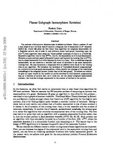
For an informal introduction to PROGRES, we will use a small specification of balanced, threaded binary trees. This well-known data structure can be used for search and sorting problems with variable data. We use this data structure as an example in order to show that its PROGRES specification has the same time complexity as an implementation in any other language e.g. like C. For the definition of basic operations on diane graphs, PROGRES provides its users with means for the construction of graph rewriting rules (productions and tests) and derived relations on nodes (paths and restrictions). Figure 1 shows an example tree in the form of a directed, attributed, node- and edge-labelled graph (diane graph). We now try to insert a new element 9 into this tree. This will be done by the production call TBTInsertLeft( Anchor, 9 ). Figure 2 shows the declaration of the production TBTInsertLeft. Applying this production to the graph in Figure 1 works as follows: 4 AnchorNode Root
5 Value: 7
n
n
l
r n
2 Value: 4
l
1 Value: 2
n
n
n
r
3 Value: 5
Figure 1: An example threaded binary tree
6 Value: 10
n
r
7 Value: 11
4
node class Node intrinsic Value : integer ; end; node type AnchorNode : Node end; node type TreeNode : Node end; edge type Root : Node [0:1] -> Node [0:1]; edge type l : Node [0:1] -> Node [0:1]; edge type r : Node [0:1] -> Node [0:1]; edge type n : Node [0:1] -> Node [0:1]; production TBTInsertLeft ( Anchor : Node ; NewVal : integer ) = ‘3
Find(NewVal)
‘2
n
: TreeNode
: TreeNode
‘1 = Anchor
not with -l-> ::= 3’ = ‘3
2’ = ‘2
n
l
1’ = ‘1
n
4’ : TreeNode condition (‘3. Value < NewVal) and (NewVal < ‘2. Value); transfer 4’.Value := NewVal; end; path Find ( NewVal : integer ) : Node -> Node [0:1] = -Root-> & { valid (NewVal < self. Value) & -l-> | valid (NewVal > self. Value) & -r-> } end;
Figure 2: Parts of the specification of TBTrees 1. First of all, a (partial) subgraph of the current work graph which is isomorphic to the graph on the left-hand side of the production is determined, i.e. a subgraph consisting of three nodes, one of type AnchorNode (‘1) and two nodes of type TreeNode (‘2 and ‘3). The nodes matched by ‘2 and ‘3 have to be connected by an edge labelled n which builds the thread. The restriction “not with -l->” to node ‘2 ensures that the matched node not already has an outgoing edge labelled l connecting it to a left son. The first parameter of TBTInsertLeft, Anchor, is used to pass the internal reference for the node to be matched by ‘1 (in our example in Figure 1 this is the key number 4)1. The assignment “= Anchor” within node ‘1 directly matches this node to the node with the corresponding key in our data 1. This internal key is returned by the production TBTCreate as out parameter.
5
structure. From node ‘1, the derived relation (in PROGRES called path) “Find( NewVal )” leads to node ‘2 (i.e. the matched nodes 4 and 6 in Figure 1). The path Find is also defined in Figure 2. From the start node (which is an implicit parameter to the path) first an edge labelled Root is traversed. This part of the path is concatenated by & to an iteration enclosed by { }. The iteration consists of two alternative parts. If the parameter NewVal is less than the Value attribute of the current node (denoted by self), and an outgoing edge labelled l exists, then this edge is traversed. Else ( | ), if NewVal is greater than the current value and an r-edge exists, we walk down to the right son. This is iterated until all (i.e. both) alternatives fail. Then the current start node of the iteration is the computed result1. So the path Find( 9 ) in our example leads from the Anchor node 4 via the Root edge to node 5 and via the second alternative to the final node 6, the insertion point for our new tree element. Finally, the attribute condition “‘3.Value < NewVal < ‘2.Value” ensures that we really found the correct insertion place2. 2. When a matching subgraph of the current work graph has been selected, this subgraph is removed from the work graph and the graph on the right-hand side of the production is inserted. A node inscription like “2’ = ‘2” designates an identical replacement of a node by itself. This means that 2’ is the same node as ‘2 and all its attribute values and all incoming or outgoing edges remain unchanged unless they are explicitly mentioned within the production. So the production removes only the n-edge connecting the nodes that are matched against ‘3 and ‘2. A new node of type TreeNode is created and connected to the remaining graph by two n-edges and the l-edge. Finally the transfer instruction is executed, assigning NewVal to the Value-attribute of the newly created node. One possible result graph of an application of TBTInsertLeft( Anchor, 9) to the graph in Figure 1 is shown in Figure 3. We hope that this short introduction to PROGRES suffices to give an impression of the language and its operations as well as the task to execute a PROGRES production. The rest of the paper concentrates on matching the left-hand side of a production to an isomorphic image within the current work graph.
3
The search plan space
The most general strategy for matching the left-hand side of a production works as follows: First, we compute the sets of candidates for all left side nodes (by querying our database for the sets of all nodes of the corresponding types). Then, for every left side node we choose a current candidate. Finally, we check our choices for fullfilling all remaining edge, path and attribute requirements of the left-hand side. If any of these requirements fails, we have to try another combination of candidates for the left-side nodes. This is repeated until all requirements are met (and an matching subgraph is found) or until all combinations failed (the searched subgraph doesn´t exist). While this standard search strategy could be used for any production, it is not very efficient since it does not utilize any of the advanced querying possiblities and indexing schemes of our underlying database management system GRAS. Often, it is possible to determine a left-side 1. Note that, in general, traversing an edge may yield a set of nodes and the iteration will be considered for each element of this set, so the iteration computes a set of nodes as result. Note also that cyclic iterations are detected and terminated automatically (cf. [Schürr 91]). 2. This attribute condition is added only for demonstration purposes, since in a correct structured search tree, the construction of our left-hand side and of the path Find already ensure the correct insertion point.
6
4 AnchorNode Root
5 Value: 7
n l
2 Value: 4 l
1 Value: 2
n
n
r
n
r
3 Value: 5
n
6 Value: 10
n
l
8 Value: 9
n
n
r
7 Value: 11
Figure 3: The resulting tree of applying TBTInsertLeft(Anchor, 9) to the tree of Figure 1 node by evaluating it´s initial assignment. Once a candidate is chosen for a left-side node, its neighbours could easily be determined by traversing the corresponding left-side edges. Inspecting attribute conditions and other restrictions as early as possible we often could avoid the costs of query actions for non matching canditate combinations. In general there is a huge number of alternative action sequences that could be used to match the left-hand side of a given graph rewriting rule. So, the central problem in executing a graph rewriting rule is to find a sequence of basic query actions that matches the left-hand side with a good or optimal efficiency. In this chapter we first model the left-hand side of a production as a diane graph. Then we consider possible query actions for matching the different elements of a left-hand side and their interdependencies. Therefore, we enrich the diane graph built for the left-hand side of a production by action nodes (representing the query actions) which are connected to the parts of the left-hand side graph they are dealing with. Once we have built the graph modelling all elements of the left-hand side of our production and all query actions that may be used to match these elements, this action graph will be used to derive a sequence of query actions that match the whole left-hand side to (one of) its isomorphic image(s) within the current work graph as efficiently as possible. Within the PROGRES environment, a production is stored as an abstract syntax tree enriched by context sensitive edges comprising symbol table information (cf. [Lewe 88, Koss 92]). For our purposes a simpler representation suffices, reducing the structure of left-hand side elements to a single node with a text attribute containing the corresponding specification part. The example production TBTInsertLeft is represented by the left-hand side graph shown in Figure 4. The left-hand side of TBTInsertLeft is modelled by one node for every node to be matched by the left-hand side, one node for every initial assignment, restriction and attribute condition, and one node for every required edge and path. The interdependencies of the lefthand side elements are represented by edges of the types:
7
= Anchor
LSfs
‘1:AnchorNode
LSfs
Find( NewVal)
LStt
not with -l->
LSfs
‘2:TreeNode
LSarg
LStt
‘3.Val left side edge, path , or restriction.
2. LStt : left side edge or path -> left side node 3. LSarg :left side restriction or attribute condition -> left side node LSfs-edges lead from a left side node to a left side edge, path, or restriction that uses it as source node. LStt-edges lead from left side edges or paths to their target nodes. LSarg-edges lead from
a left side restriction or attribute condition to left side nodes that are used as arguments. E. g., in Figure 4 the node “ ‘2 : TreeNode” is • target of a LStt-edge from the path “Find( NewVal )”, • source of a LSfs-edge leading to the node “-n->”, • source of a LSfs-edge leading to the restriction “not with -l->”, • target of a LSarg-edge from the attribut condition “ ‘3.Val” node of Figure 4 a TestRestriction node is generated, with one1 r-edge leading to “‘2:TreeNode” and with an m-edge leading to “not with -l->”, cf. Figure 11. For a left side attribute condition nearly the same graph rewriting rule is used. Instead of a TestRestriction action a TestAttCond action is created. Since an attribute condition has no incoming LSfs-edge the corresponding left side node is omitted, cf. Figure 5. By applying this left side restriction LSarg
left side restriction
=>
left side left side restriction node
LSarg
left side left side restriction node
m r
TestAttCond
Figure 6: Action for left side attribute conditions rule to the attribute condition “‘3.Val
r m
r TestNodeExpr
r
left side left side restriction node
left side left side restriction node
left side node
m
GetNodeExpr
Figure 7: Action for left side node expressions matches both left side elements, the node and the corresponding expression (cf. node “= Anchor” in Figure 10). A left side edge may be matched by three different actions. If source and target nodes are already matched, we only have to test the existence of the required edge. On the other hand, if only one of the connected left side nodes already has been found until now, we could traverse the edge in forward or reverse direction using the actions GetTargets or GetSources respectively. Cf. Figure 8 and node “-n->” of Figure 11. left side node
r
left side node
LSfs
r
LSfs
m
GetSources
m left side edge LStt
=>
TestEdge
m
r
left side edge
m
LStt m
left side node
left side node
GetTargets
r
Figure 8: Action for left side edges The next operation for our action graph generates a GetPath and a TestPath action for left side paths. Note that there is no GetSourcesOfPath action available since, unlike edges, we are not able to traverse paths against their declared direction. So, left side paths are handled like left side edges, just omitting the GetSources action and using the path actions instead of the edge actions, cf. node “Find( NewVal)” of Figure 11. Finally, in Figure 10, the most general action that can be used to match a left side node is modelled. We are always able to match a left side node by querying for all nodes of a certain type. This query action should be used only as a last resort, since in general it computes a very large set of nodes. Note that the GetInstances action always computes a set of nodes as result. Other Get actions like the GetTargets action for traversing an edge in general also compute a set of nodes. But, considering our example of Figure 2 again, we see that for all nodes of the tree there exists at most one outgoing edge of a given edge type. Thus, traversing e.g. an l-edge will compute at most one node. It is very important for our matching strategy to be able to divide the Get actions into set valued actions, which compute a set of nodes, and into element valued
10
actions that compute at most one node. Thus we augmented the declarations of edge types (and paths) in PROGRES by an optional cardinality assertion. The declarations edge_type E1 : Node -> Node [0:1] ; edge_type E2 : Node -> Node [1:1] ; edge_type E3 : Node -> Node [0:n] ; edge_type E4 : Node -> Node [1:n] ;
ensure that for every node in the specified graph holds that there exists at most one outgoing E1-edge, exactly one outgoing E2-edge, any number of E3-edges, and at least one E4-edge. The same cardinality assertions may be made for the source types, cf. Figure 2. To be able to make use of this cardinality information for our matching strategies, we introduce an additional left side candidates node for every left side node, modelling the results of set valued actions. A candidates node represents a set of candidates for matching the corresponding left side node. A GetSelection action is used to loop through the set of candidates. The original left side node represents the actual choice for matching this left side node to a node of the current work graph. Thus, the GetSelection action requires the candidates node and matches the corresponding left side node representing the current selection. m
left side candidates
=>
left side node
GetInstances
r m
left side node
GetSelection
Figure 9: Actions for left side nodes At this point we have to refine all previous actions to reflect the distinction of set and element valued Get actions. Set valued actions will match only the candidates node, while element valued actions directly match both the candidates and the corresponding left side node. Instead, we use the action of Figure 10 to (1) remove all m-edges connecting a set valued Get action with the original left side node, and (2) to insert new m-edges connecting the set valued and the element valued Get actions to the candidates node. left side candidates
GetGetInstances Action
GetGetInstances Action
m
left side candidates
r GetSelection
IsSetValued m GetGetInstances Action
m
r
=>
GetSelection
m left side node
m GetGetInstances Action
m
m left side node
IsElemValued
Figure 10: Splitting set and element valued Get actions Applying all these operations (using the one of Figure 10 as the last) to the graph of Figure 4 leads to the action graph for TBTInsertLeft shown in Figure 11. Note that in our example speci-
11
m
m
GetNodeExpr
m r LSfs
= Anchor
GetSelection
‘1:AnchorNode
‘1 Candidates
m m
r
TestNodeExpr
GetInstances r
m
r LSfs
TestPath
GetPath
Find( NewVal) m
m LStt r
m
TestRestriction
m
m
r m
not with -l->
GetSelection
‘2:TreeNode
LSfs
r ‘2 Candidates GetInstances
m m
r LSarg TestAttCond
m
r
r
LStt
‘3.Val