systems Article
A Hierarchical Aggregation Approach for Indicators Based on Data Envelopment Analysis and Analytic Hierarchy Process Mohammad Sadegh Pakkar Received: 24 November 2015; Accepted: 12 January 2016; Published: 20 January 2016 Academic Editor: Hong Wang Faculty of Management, Laurentian University, Sudbury, ON P3E 2C6, Canada;
[email protected]; Tel.: +1-705-675-1151
Abstract: This research proposes a hierarchical aggregation approach using Data Envelopment Analysis (DEA) and Analytic Hierarchy Process (AHP) for indicators. The core logic of the proposed approach is to reflect the hierarchical structures of indicators and their relative priorities in constructing composite indicators (CIs), simultaneously. Under hierarchical structures, the indicators of similar characteristics can be grouped into sub-categories and further into categories. According to this approach, we define a domain of composite losses, i.e., a reduction in CI values, based on two sets of weights. The first set represents the weights of indicators for each Decision Making Unit (DMU) with the minimal composite loss, and the second set represents the weights of indicators bounded by AHP with the maximal composite loss. Using a parametric distance model, we explore various ranking positions for DMUs while the indicator weights obtained from a three-level DEA-based CI model shift towards the corresponding weights bounded by AHP. An illustrative example of road safety performance indicators (SPIs) for a set of European countries highlights the usefulness of the proposed approach. Keywords: data envelopment analysis; analytic hierarchy process; composite indicators; hierarchical structures; indicator weights
1. Introduction Individual indicators are multidimensional measures that can assess the relative positions of entities (e.g., countries) in a given area [1]. A Composite indicator (CI) is a mathematical aggregation of individual indicators into a single score. Two simple but popular aggregation methods in the context of multi-criteria decision-making (MCDM) are the weighted sum (WS) method and the weighted product (WP) method [2]. Some researchers have recently pointed out that the WP method may have some advantages over the WS method in CI construction [3–5]. However, the assignment of weights to indicators is still a main source of difficulty in the application of these methods. Fortunately, the recent methodological advances in operations research and management science (OR/MS) have provided us with two powerful tools, namely data envelopment analysis (DEA) and analytic hierarchy process (AHP), which can be used as weighting and aggregation tools in CI construction. Data Envelopment Analysis is a nonparametric method to assess the relative efficiency of a group of DMUs based on their distance from the best-practice frontier. In this method each DMU can freely choose its own weights to maximize its performance [6]. The standard DEA models are formulated using multiple inputs and multiple outputs of DMUs. The application of this group of models in CI construction can be found in [7–9]. However, in recent years much more attention has been focused on the application of a new group of DEA models in the field of composite indicators which is known as the “benefit of the doubt” (BOD) approach. Systems 2016, 4, 6; doi:10.3390/systems4010006
www.mdpi.com/journal/systems
Systems 2016, 4, 6
2 of 17
In the BOD approach, all indicators are treated as outputs without explicit inputs, i.e., the property of “the larger is the better” [10–12]. In light of the possibility of neglecting the priority of various indicators, some critics have questioned the validity and stability of CIs obtained via DEA. Decision makers (DMs), in some contexts, have value judgments concerning the relative priority of indicators that should be taken into account in CI construction. Alternatively, AHP is a systematic MCDM method to generate the true or approximate weights based on the well-defined mathematical structures of pairwise comparison metrics. The application of AHP in CI construction provides a priori information about the relative priority of indicators [13–15]. AHP usually involves three basic functions: structuring complexities, measuring on a ratio-scale and synthesizing [16]. One of the advantages of AHP is its high flexibility to be combined with the other OR/MS techniques [17]. AHP can be combined with DEA in different ways. The most common approach is the estimation of parameters of weight restrictions on the DEA models. AHP estimates the appropriate values for the parameters in the absolute weight restrictions [18], relative weight restrictions [19–23], virtual weight restrictions [24,25] and restrictions on changes of input (output) units [26]. There are a number of other methods that do not necessarily apply additional restrictions to a DEA model. Such as converting the qualitative data in DEA to the quantitative data using AHP [27–34], ranking the efficient/inefficient units in DEA models using AHP in a two stage process [35–37], weighting the efficiency scores obtained from DEA using AHP [38], weighting the inputs and outputs in the DEA structure [39–42], constructing a convex combination of weights using AHP and DEA [43] and estimating missing data in DEA using AHP [44]. The recent studies by Pakkar [45–50] demonstrate the effects of imposing weight bounds on the different variants of DEA models using AHP. To this end, AHP has been applied in single-level DEA models [47–50] and two-level DEA models [45,46]. Due to the complexity of the hierarchical structures of indicators, this paper applies AHP into an additive three-level DEA model in the context of CI construction. Theoretically, the approach proposed in this paper may also be considered as the additive form of the multiplicative three-level DEA-based CI approach to constructing CIs proposed by [51]. In a three-level hierarchy, the indicators of similar characteristics can be grouped into sub-categories and further into categories. A three-level DEA model entirely reflects the characteristics of a generalized multiple level DEA model developed in [52,53]. Since the proposed approach uses AHP in an additive three-level DEA-based model, it contributes to the set of methods currently available for CI construction. 2. Methodology This research has been organized to proceed along the following stages (Figure 1): 1. 2. 3. 4. 5.
Computing the composite value of each DMU using one-level DEA-based CI model (4). The computed composite values are applied in three-level DEA-based CI model (6). Computing the priority weights of indicators for all DMUs using AHP, which impose weight bounds into model (6). Obtaining an optimal set of weights for each DMU using three-level DEA-based CI model (6) (minimum composite loss η). Obtaining an optimal set of weights for each DMU using model (6) bounded by AHP (maximum composite loss κ). Note that if the AHP weights are added to model (6), we obtain model (10). Measuring the performance of each DMU in terms of the relative closeness to the priority weights of indicators. For this purpose, we develop parameter-distance model (11). Increasing a parameter in a defined range of composite loss we explore how much a DM can achieve its goals. This may result in various ranking positions for a DMU in comparison to the other DMUs.
Systems 2016, 4, 6 Systems 2016, 4, x
3 of 17 3 of 17
Figure 1. 1. A A hierarchical hierarchical aggregation aggregation approach approach for for indicators indicators using using aa three-level three-level Data Data Envelopment Envelopment Figure Analysis (DEA) and Analytic Hierarchy Process (AHP). Analysis (DEA) and Analytic Hierarchy Process (AHP).
2.1. DEA-Based 2.1. DEA-Based CI CI Model Model A DEA-based CI model can be similar to to aa classical A DEA-based CI model can be formulated formulated similar classical DEA DEA model model in in which which all all data data are are treated as outputs without explicit inputs [54]. In the following, and in line with the more common treated as outputs without explicit inputs [54]. In the following, and in line with the more common CI CI terminology, we often will often refer to outputs as “indicators”. order to the eliminate the scale terminology, we will refer to outputs as “indicators”. In order In to eliminate scale differences differences (output) indicators, and moreover, to ensure that allare of in them in direction the same between allbetween (output)all indicators, and moreover, to ensure that all of them the are same direction of change the normalized counterparts of indicators, using the distance to reference method, of change the normalized counterparts of indicators, using the distance to reference method, are are computed as follows [1]: computed as follows [1]:
yˆ
yˆrjrj , yˆ max{ yˆ r1 , yˆ r 2 ,..., yˆ rn} for desirable indicators yrjyrj“ ˆ , yˆrrp(max) maxq “ max tyˆ r1 , yˆ r2 , ..., yˆ rn u for desirable indicators yˆryprmax (max) q
(1) (1)
yˆryˆpmin r (min) q ˆˆr2 ˆˆrrp(min) , , yy “min{ min tyˆyˆrr1 ..., yˆyˆrnrnu} for undesirable indicators yrjyrj“ minq 1 ,, y r 2,,..., yˆyrj ˆ
(2) (2)
rj
where yrj is the normalized value of (output) indicator r (r “ 1, 2.., s) for DMU j (j = 1, 2, . . . , n). where yrj is the normalized value of (output) indicator r ( r 1, 2.., s ) for DMU j ( j 1, 2,..., n ). Now assume that all DMUs have unit input i (i “ 1, 2, ..., m). Then the fractional CCR-DEA model can Now assume that all DMUs be developed as follows [55]:have unit input i ( i 1, 2, ..., m ). Then the fractional CCR-DEA model s ř can be developed as follows [55]: ur yrk r“s1 Max CIk “ m (3) ř uvr iyrk Max CI k ri“1m1 (3) s ř vi ur yrj i 1 r“1 ď 1 @j m ř v i s
i“1 u y u ,v ą 0 r r r1 i m
rj
1@r,i j
where CIk is the composite indicator of DMU under assessment. k is the index for the DMU under vi assessment where k ranges over 1, 2, . . . , n.i v1 i and ur are the weights of input i (i “ 1, 2, ..., m) and (output) indicator r (r “ 1, 2.., s). The first set of constraints assures that if the computed weights 0 r , i do not attain a composite score of larger are applied to a group of n DMUs, (j “ 1,ur2,, v..., they i >n), than 1. The second set of constraints indicates the non-negative conditions for the model variables. where CI k is the composite indicator of DMU under assessment. k is the index for the DMU under
assessment where
k ranges over 1, 2,…, n . vi and u r are the weights of input i ( i 1, 2,..., m )
and (output) indicator r ( r 1, 2.., s ). The first set of constraints assures that if the computed weights are applied to a group of
n
DMUs, ( j 1, 2,..., n ), they do not attain a composite score of larger
than 1. The second set of constraints indicates the non-negative conditions for the model variables.
Systems 2016, 4, 6
4 of 17
Introducing the constraint
m ř
vi “ 1 and performing the operation of substitution, an equivalent
i “1
linear model can be formulated as follows: CIk “
Max
s ÿ
ur yrk
(4)
r “1 s ÿ
ur yrj ď 1
@j
r“1
ur ą 0
@r.
Model (4) looks like a DEA model without inputs that extends the standard DEA methodology to the field of CI construction. 2.2. Three-Level DEA-Based CI Model We develop a three-level DEA model to aggregate the performance of indicators under the (sub) category they belong to by a weighted-average method (Figure 2). Let yll 1 rj be the value of indicator r (r “ 1, 2, ..., s) of sub-category l 1 pl 1 “ 1, 2, ..., S1 q of category l pl “ 1, 2, ..., Sq for DMU j (j “ 1, 2, ..., n) after normalizing the original data. Let ull 1 r be the internal weight of indicator r of sub-category l 1 s ř ull 1 r “ 1. Then the value of sub-category l 1 of category l for the DMU j is of category l while r “1
defined as yll 1 j “ S1 ř l 1 “1
p
ll 1
s ř
r“1
ull 1 r yll 1 rj . Let pll 1 be the internal weight of sub-category l 1 of category l while
“ 1. Then the value of category l is defined as ylj “
S1 ř l 1 “1
pll 1 yll 1 j . Let pl be the weight of
category l. To develop a linear model, the new multiplier of indicator r of sub-category l 1 of category l is defined as: u1ll 1 r “ pl pll 1 ull 1 r . Similarly, the new multiplier of sub-category l 1 of category l is defined as: p1 ll 1 “ pl pll 1 . Consequently, a linear three-level DEA model for indicators can be developed as follows: S ÿ S1 ÿ s ÿ Max CIk “ u1ll 1 r yll 1 rk (5) l “1 l 1 “1 r“1 1
S ÿ S ÿ s ÿ
u1ll 1 r yll 1 rj ď 1
@j
l “1 l 1 “1 r “1 1
S ÿ s ÿ
u1ll 1 r “ pl
@l
l 1 “1 r“1 s ÿ
u1ll 1 r “ p1ll 1
@l, l 1
r “1
u1ll 1 r , p1ll 1 , pl
ą0
@l, l 1 , r.
Systems 2016, 4, 6 Systems 2016, 4, x
5 of 17 5 of 17
Figure for hierarchical hierarchical indicators. indicators. Figure 2. 2. A A three-level three-level DEA DEA framework framework for
We develop our formulation based on the generalized distance model [56,57] in such a way that We develop our formulation based on the generalized distance model [56,57] in such a way the hierarchical structures of indicators, using a weighted-average approach, are taken into that the hierarchical structures of indicators, using a weighted-average approach, are taken into * CI consideration [52,53]. Let ( be the the best best attainable attainable composite composite value value for for the the DMU DMU ˚ 1,22,,..., n ) be consideration [52,53]. Let CIkk (kk“ 1, ..., n) 1 under assessment, calculated calculated from from model model (4). (4). We Wewant wantthe thecomposite compositevalue value CI CIkk pu (ull 1rr)q,, calculated 1 ˚ from the set of weights ull 1 r , to be closest to CIk* . The degree of closeness between CIk pu1ll 1 r q and from the set of weights ull r , to be closest to CI k . The degree of closeness between CI k (ull r ) and t 1{t CIk˚* is measured as Dt “ rCIk˚* ´ CIk pu1ll 1 r q ts 1/ t with t ě 1, where Dt is a distance measure and t CI k is measured as Dt [CI k CI k (ull r ) ] with t 1 , where Dt is a distance measure and t represents the distance parameter. Our definition of “closest” is that the largest distance is at its represents Our definition “closest” dominates is that the when largestt distance minimum. the On distance the otherparameter. hand, the largest distance of completely “ 8. Forist at “ its 8, ( t t , minimum. On the other hand, the largest distance completely dominates when . For ˚ 1 the distance measure is reduced to D8 “ max CIk ´ CIk pull 1 r q . Hence we choose the form of the * u1ll 1 r the distance measure is reduced to D max{ ( CI k CI k (ull r )} . Hence we choose the form of the ˚ 1 u ll r minimax model: min max CIk ´ CIk pull 1 r q to minimize a single deviation which is equivalent to u1ll 1 r k“1,...,n max{CI k* CI k (ull r )} to minimize a single deviation which is equivalent to minimax model: min the following linearullmodel: r k 1,..., n Min η (6) the following linear model: S ÿ S ÿ ÿ Mins 1 ´ ull 1 r yll 1 rk ď η 1
CIk˚
(6)
l “1 l 1 “1 r“1 S
S
s
u y u1 y ď CI ˚ @j
SCIÿ S s ÿ k ÿ *1
ll r l 1 l ll 11 r r ll11 rj
ll rk
j
l “1 l 1 “1 r “1 S 1 s S ÿ s ÿ r 1 1ll rj“ ll u ll r l 1 l 11 r 1 S
u
y
* pCI @l j j
l
l “1 r“1
sS ÿ
s 1 1 u1ll 1 ru“ pll1 p @l,l l
rl“ 11 r 1
ll r
u1ll 1 r , p1ll 1 , pl ą 0 s
u r 1
ll r
l
@l, l 1 , r
ηěp0. ll l , l
Model (6) identifies the minimum composite loss η (eta) needed to arrive at an optimal set of weights. The first constraint ensures ull rthat , pll each , pl DMU 0 lloses , l , r no more than η of its best attainable composite value, CIk˚ . The second set of constraints satisfies that the composite values of all DMUs are less than or equal to their upper bound of CIj˚ .
0.
Model (6) identifies the minimum composite loss
(eta) needed to arrive at an optimal set of
weights. The first constraint ensures that each DMU loses no more than
of its best attainable
Systems 2016, 4, x
composite value,
6 of 17
CI k* . The second set of constraints satisfies that the composite values of all DMUs
Systems 2016, 4, 6
are less than or equal to their upper bound of
6 of 17
CI *j . S
s
s
Two sets of constraints are added to model (6): us ll r pl and uř S1 ř s r pll , where ull r are ř ll r 1 Two sets of constraints are added to model (6): l 1 r 1 u1ll 1 r “ pl and u1ll 1 r “ p1ll 1 , where u1ll 1 r 1 “1 r “1 r “ 1 l indicator multipliers. This implies that the sum of weights under each (sub-) sub-category equals to are indicator multipliers. This implies that the sum of weights under each (sub-) sub-category equals the weight of that (sub-) sub-category. It should be noted that the original (or internal) weights used to the weight of that (sub-) sub-category. It should be noted that the original (or internal) weights used for andp p1 ll“ uull1 r {pp1ll and p1p ll pl . forcalculating calculatingthe theweighted weightedaverages averagesare are obtained obtained as as uullll1rr “ ll ll 1 r ll 1 ll 1 {pl . 2.3. 2.3.Prioritizing PrioritizingIndicator IndicatorWeights WeightsUsing UsingAHP AHP Model Model(6) (6)identifies identifiesthe theminimum minimumcomposite compositeloss lossη (eta) needed to arrive at at aa set set of of weights weightsof of indicators by the internal mechanism of DEA. On the other hand, the priority weights of indicators, indicators by the internal mechanism of DEA. On the other hand, the priority weights of indicators, andthe thecorresponding corresponding(sub) (sub)categories categoriesare aredefined definedout outof ofthe theinternal internalmechanism mechanismof ofDEA DEAby byAHP AHP and (Figure 3). (Figure 3).
Figure3.3.The TheAHP AHPmodel modelfor forprioritizing prioritizingindicators. indicators. Figure
In how AHP is integrated into thethe three-level DEA-based CI Inorder ordertotomore moreclearly clearlydemonstrate demonstrate how AHP is integrated into three-level DEA-based model, this research presents an analytical process in which indicator weights are bounded by the CI model, this research presents an analytical process in which indicator weights are bounded by AHP method. The The AHP procedure for for imposing weight bounds may bebebroken the AHP method. AHP procedure imposing weight bounds may brokendown downinto intothe the following steps: following steps: Step pairwise comparison comparisonmatrix matrixofofdifferent differentcriteria, criteria,denoted denoted Step 1: 1: A A decision decision maker makes aa pairwise byby A, ( l q 1, 2,..., S ) A , with the entries . The comparative importance of criteria is provided with the entries of alqofpl a“ q “ 1, 2, ..., Sq. The comparative importance of criteria is provided by the lq decision maker using a rating scale. Saaty recommends using ausing 1–9 scale. by the decision maker using a rating scale. [16] Saaty [16] recommends a 1–9 scale. Step 2: The AHP method obtains the priority weights of criteria bycomputing computingthe theeigenvector eigenvectorof of Step 2: The AHP method obtains the priority weights of criteria by T matrix A (Equation (7)), w “ pw , w , ..., w q , which is related to the largest eigenvalue, λmax . T matrix A (Equation (7)), w (1w1 ,2w2 ,...,SwS ) , which is related to the largest eigenvalue, max . Aw λmaxw w Aw “
(7)(7)
max
To determine whether or not thethe inconsistency inina acomparison the random random To determine whether or not inconsistency comparisonmatrix matrixis is reasonable reasonable the consistency ratio, C.R., can be computed by the following equation: consistency ratio, C.R. , can be computed by the following equation: λmax ´ N C.R. “ max N C .R. pN ´ 1qR.I. (N 1) R.I .
(8) (8)
where R.I. is the average random consistency index and N is the size of a comparison matrix. where R.I . is the average random consistency index and N is the size of a comparison matrix. In a In a similar way, the priority weights of (sub-) sub-criteria under each (sub-) criterion can be computed. similar way, the priority weights of (sub-) sub-criteria under each (sub-) criterion can be computed. To obtain the weight bounds for indicator weights in the three-level DEA-based CI model, this study To obtain the weight bounds for indicator weights in the three-level DEA-based CI model, this study aggregates the priority weights of three different levels in AHP as follows: aggregates the priority weights of three different levels in AHP as follows: ull 1 r “ wl ell 1 f ll 1 r ,
S ÿ l “1
1
wl “ 1,
s ÿ l 1 “1
ell 1 “ 1
and
s ÿ r“1
f ll 1 r “ 1
(9)
Systems 2016, 4, 6
7 of 17
where wl is the priority weight of criterion l (l “ 1, ..., S) in AHP, ell 1 is the priority weight of sub-criterion l 1 pl 1 “ 1, 2, ..., S1 q under criterion l and f ll 1 r is sub-sub-criterion r (r “ 1, ..., s) under sub-criterion l 1 . In order to estimate the maximum composite loss κ (kappa) necessary to achieve the priority weights of indicators for each DMU the following linear program is proposed: Min
(10)
κ
u1ll 1 r “ αull 1 r
@l, l 1 , r
1
CIk˚ ´
S ÿ s S ÿ ÿ
u1ll 1 r yll 1 rk ď κ
l “1 l 1 “1 r “1 1
S ÿ s S ÿ ÿ
u1ll 1 r yll 1 rj ď CIj˚
@j
l “1 l 1 “1 r “1 1
S ÿ s ÿ
u1ll 1 r “ pl
@l
l 1 “1 r “1 s ÿ
u1ll 1 r “ p1ll 1
@l, l 1
r “1
u1ll 1 r , p1ll 1 , pl κ ě 0,
ą0
@l, l 1 , r
α ą 0.
The first sets of constraints change the AHP computed weights to weights for the new system by means of a scaling factor α. The scaling factor α is added to avoid the possibility of contradicting constraints leading to infeasibility or underestimating the relative composite scores of DMUs [58]. The optimal solution to model (10) produces a set of weights for indicators that are used to compute the performance of DMUs. It should be noted that incorporating absolute weight bounds, using AHP, for indicator weights in a DEA-based CI model is consistent with the common practice of constructing composite indicators. According to this practice, the priority weights of indicators can be used directly in an aggregation function to synthetize indicators’ values into composite values [1]. In addition, this form of placing restrictions on indicator weights simply allows us to identify a specific range of variation between two systems of weights obtained from models (6) and (10). 2.4. A Parametric Distance Model We can now develop a parametric distance model for various discrete values of parameter θ such that η ď θ ď κ. Let u1ll 1 r pθq be the weights of indicators for a given value of parameter θ, where ˚ indicators are under sub-category l 1 pl 1 “ 1, 2, ..., S1 q of category l (l “ 1, 2, ..., S). Let u1 ll 1 r pκq be the priority weights of indicators under sub-category l 1 of category l, obtained from model (10). ˚ Our objective is to minimize the total deviations between u1ll 1 r pθq and u1 ll 1 r pκq with the shortest Euclidian distance measure subject to the following constraints:
Systems 2016, 4, 6
8 of 17
˜ Min
Zk pθq “
¸1{2
1
S ÿ s S ÿ ÿ
2 ˚ pu1ll 1 r ´ u1 ll 1 r pκqq
(11)
l “1 l 1 “1 r“1 1
CIk˚
S ÿ s S ÿ ÿ
´
u1ll 1 r yll 1 rk ď θ
l “1 l 1 “1 r “1 1
S ÿ S ÿ s ÿ
u1ll 1 r yll 1 rk ď θ ď CIj˚
@j
l “1 l 1 “1 r“1 1
S ÿ s ÿ
u1ll 1 r “ pl
@l
l 1 “1 r“1 s ÿ
u1ll 1 r “ p1ll 1
@l, l 1
r “1
u1ll 1 r , p1ll 1 , pl ą 0
@l, l 1 , r.
Because the range of deviations computed by the objective function is different for each DMU, it is necessary to normalize it by using relative deviations rather than absolute ones [59]. Hence, the normalized deviations can be computed by: ∆k pθq “
Zk˚ pηq ´ Zk˚ pθq Zk˚ pηq
(12)
where Zk˚ pθq is the optimal value of the objective function for η ď θ ď κ. We define ∆k pθq as a measure of closeness which represents the relative closeness of each DMU to the weights obtained from model (10) in the range [0, 1]. Increasing the parameter pθq, we improve the deviations between the two systems of weights obtained from models (6) and (10) which may lead to different ranking positions for each DMU in comparison to the other DMUs. It should be noted that in a special case where the parameter θ “ κ “ 0, we assume ∆k pθq = 1. 3. A Numerical Example: Road Safety Performance Indicators In this section we present the application of the proposed approach to assess the road safety performance of a set of 13 European countries (or DMUs): Austria (AUT), Belgium (BEL), Finland (FIN), France (FRA), Hungary (HUN), Ireland (IRL), Lithuania (LTU), Netherlands (NLD), Poland (POL), Portugal (PRT), Slovenia (SVN), Sweden (SWE) and Switzerland (CHE). The data for eleven hierarchical indicators that compose SPIs for these countries have been adopted from [52]. The eight SPIs related to alcohol and speed are undesirable indicators while the three SPIs related to protective systems are desirable ones. The resulting normalized data based on Equations (1) and (2) are presented in Table 1. Taking the percentage of speed limit violation on rural roads as an example, Slovenia performs the best (1.000) while Poland the worst (0.014) and all other countries’ values lie within this interval. The results of the AHP model for prioritizing hierarchical SPIs as constructed by the author in Expert Choice software are presented in Table 2. One can argue that the priority weights of SPIs must be judged by road safety experts. However, since the aim of this section is just to show the application of the proposed approach on numerical data, we see no problem to use our judgment alone.
Systems 2016, 4, 6
9 of 17
Table 1. Normalized data on the eleven hierarchical safety performance indicators (SPIs). Alcohol
Countries
AUT BEL FIN FRA HUN IRL LTU NLD POL PRT SVN SWE CHE
% of Drivers above Legal Alcohol Limit In Roadside Police Tests
Speed Mean Speed
Protective Systems Speed Limit Violation (%)
% of Alcohol Related Fatalities
Motorways
Rural Roads
Urban Roads
Motorways
Rural Roads
0.463 0.654 0.136 0.123 0.283 0.119 0.321 1.000 0.438 0.610 0.078 0.357 0.230
0.938 0.846 0.963 0.933 0.955 0.945 1.000 0.899 0.806 0.847 0.964 0.883 0.943
0.781 0.743 0.729 0.787 0.793 0.762 0.713 0.740 0.697 0.618 1.000 0.717 0.757
0.802 0.768 0.907 0.838 0.817 0.724 0.714 0.881 0.647 0.919 0.713 0.870 1.000
0.766 0.348 0.409 0.505 0.362 1.000 0789 0.454 0.290 0.302 0.480 0.241 0.710
0.051 0.029 0.023 0.037 0.033 0.032 0.025 0.020 0.015 0.014 1.000 0.019 0.043
0.116 0.068 0.593 0.263 0.279 0.237 0.555 0.081 0.091 0.137 0.122 1.000 0.277
Child Restraint
Seat Belt
Urban Roads
Daytime Seatbelt Wearing Rate in Front Seats of Light Vehicles (%)
Daytime Seatbelt Wearing Rate in Rear Seats of Light Vehicles (%)
Daytime Usage Rate of Child Restraints (%)
0.254 0.222 0.323 0.318 0.230 0.223 0.318 0.234 0.165 0.360 0.163 0.259 1.000
0.904 0.799 0.911 1.000 0.727 0.901 0.609 0.959 0.799 0.881 0.874 0.973 0.887
0.699 0.488 0.922 1.000 0.501 0.914 0.366 0.890 0.589 0.574 0.551 0.927 0.805
0.863 0.729 0.716 0.937 0.433 0.857 0.404 0.758 0.905 0.591 0.672 1.000 0.895
Table 2. The AHP hierarchical model for SPIs. Objective Level
Criteria Level
Alcohol w1 “ 0.2727
Sub-Criteria Level
Sub-Sub-Criteria Level
% of drivers above legal alcohol limit e11 “ 0.333
% of drivers above legal alcohol limit f 111 “ 1.000
% of alcohol-related fatalities e12 “ 0.667
% of alcohol-related fatalities f 121 “ 1.000 Mean speed of vehicles on motorways f 211 “ 0.081
Mean speed e21 “ 0.60
Mean speed of vehicles on rural roads, f 212 “ 0.342 Mean speed of vehicles on urban roads, f 213 “ 0.577
Prioritizing road user behavior
Speed w2 “ 0.5454
% of vehicles exceeding the speed limit on motorways f 221 “ 0.081 Speed limit violations e22 “ 0.40
% of vehicles exceeding the speed limit on rural roads f 222 “ 0.342 % of vehicles exceeding the speed limit on urban roads f 223 “ 0.577
Seat belt e31 “ 0.40 Protective systems w3 “ 0.1818 Child Restraint e32 “ 0.60
Daytime seatbelt wearing rate in front seats of light vehicles (%) f 311 “ 0.60 Daytime seatbelt wearing rate in rear seats of light vehicles (%) f 312 “ 0.40 Daytime usage rate of child restraints (%) f 321 “ 1.000
Solving model (6) for the country under assessment, we obtain an optimal set of weights with minimum composite loss pηq. Since the raw data are normalized, the weights obtained from this model are meaningful and have an intuitive explanation. As a result, we can later set meaningful bounds on the weights in terms of the relative priority of indicators. Taking Austria as an example in Table 3, with the composite value of one obtained from model (4), we can observe that the alcohol-related fatality rate is 26 times less important than the mean speed of vehicles on motorways and about 3.2 times less important than the daytime usage rate of child restraints. Clearly, the other indicators
Systems 2016, 4, 6
10 of 17
are ignored in this assessment by assigning zero weights which are equivalent to excluding those indicators from the analysis. This kind of situation can be remedied by including the opinion of experts in defining the relative priority of indicators. Table 3. Optimal weights of hierarchical SPIs obtained from model (6) for Austria. Weights of Categories
Weights of Sub-Categories p111 p112
p1 “ 0.0361
Weights of Sub-Sub-Categories
“ 0.0000 “ 0.0361
u1111 “ 0.0000 u1121 “ 0.0361
“ 0.9415
u1211 “ 0.9415 u1212 “ 0.0000 u1213 “ 0.0000
p122 “ 0.0000
u1221 “ 0.0000 u1222 “ 0.0000 u1223 “ 0.0000
p131 “ 0.0000
u1311 “ 0.0000 u1312 “ 0.0000
p132 “ 0.1160
u1321 “ 0.1160
p121 p2 “ 0.9415
p3 “ 0.1160
η “ 0.0000
It should be noted that the composite value of all countries calculated from model (6) is identical to that calculated from model (4). Therefore, the minimum composite loss for the country under assessment is η “ 0 (Table 4). This implies that the measure of relative closeness to the AHP weights for the country under assessment is ∆k pηq “ 0. On the other hand, solving model (10) for the country under assessment, we adjust the priority weights of hierarchical SPIs obtained from AHP in such a way that they become compatible with the weights’ structure in the three level DEA-based CI models. Table 5 presents the optimal weights of hierarchical SPIs as well as its scaling factor for all countries. Table 4. Minimum and maximum losses in composite values for each country. Countries
CIk ˚
η
κ
AUT BEL FIN FRA HUN IRL LTU NLD POL PRT SVN SWE CHE
1.000 0.938 1.000 1.000 1.000 1.000 1.000 1.000 0.955 0.978 1.000 1.000 1.000
0.000 0.000 0.000 0.000 0.000 0.000 0.000 0.000 0.000 0.000 0.000 0.000 0.000
0.158 0.127 0.173 0.184 0.284 0.254 0.270 0.023 0.224 0.139 0.208 0.040 0.000
Systems 2016, 4, 6
11 of 17
Table 5. Optimal weights of hierarchical SPIs obtained from model (10) for all countries. Weights of Categories
Weights of Sub-Categories p111 p112
p1 “ 0.4089
Weights of Sub-Sub-Categories
“ 0.1362 “ 0.2727
u1111 “ 0.1362 u1121 “ 0.2727
p121 “ 0.4907
u1211 “ 0.0397 u1212 “ 0.1678 u1213 “ 0.2831
p122
“ 0.3271
u1221 “ 0.0265 u1222 “ 0.1119 u1223 “ 0.1888
p131 “ 0.1090
u1311 “ 0.0654 u1312 “ 0.0436
p132 “ 0.1636
u1321 “ 0.1636
p2 “ 0.8178
p3 “ 0.2726
α “ 1.4993
Note that the priority weights of AHP used for incorporating weight bounds on indicator weights u1 1 in model (10) are obtained as ull 1 r “ ll r . Similarly, the priority weights of AHP at criteria level α S1 ř s s ř ř pl u1ll 1 r “ pl and u1ll 1 r “ p1ll 1 . In addition, The priority can be obtained as wl “ while α r “1 l 1 “1 r “1 weights of AHP at sub-criteria and sub-sub-criteria levels can be obtained as ell 1 “ p1ll 1 {pl and f ll 1 r “ u1ll 1 r {p1ll 1 , respectively. The maximum composite loss for each country to achieve the corresponding weights in model (10) is equal to κ (Table 4). As a result, the measure of relative closeness to the priority weights of SPIs for the country under assessment is ∆k pκq = 1. Going one step further to the solution process of the parametric distance model (11), we proceed to the estimation of total deviations from the AHP weights for each country while the parameter θ is 0 ď θ ď κ. Table 6 represents the ranking position of each country based on the minimum deviation from the priority weights of indicators for θ “ 0. It should be noted that in a special case where the parameter θ “ κ “ 0 we assume ∆k pθq “ 1. Table 6. The ranking position of each country based on the minimum distance to priority weights of SPIs. Countries
Z ˚ p ηqq
Rank
AUT BEL FIN FRA HUN IRL LTU NLD POL PRT SVN SWE CHE
0.332 0.705 0.438 0.338 0.591 0.331 0.381 0.021 0.718 0.782 0.166 0.035 0.000
6 11 9 7 10 5 8 2 12 13 4 3 1
Table 6 shows that Switzerland (CHE) is the best performer in terms of the CI value and the relative closeness to the priority weights of indicators in comparison to the other countries. Nevertheless, increasing the value of θ from 0 to κ has two main effects on the performance of the other countries: improving the degree of deviations and reducing the value of composite indicator. This, of course,
Systems 2016, 4, 6 Systems 2016, 4, x
12 of 17 12 of 17
( )4, indicator. This, of course, is a phenomenon, one expects to observe frequently. The graphinofFigure is a phenomenon, one expects to observe frequently. The graph of ∆pθq versus θ, as shown versus shownthe in relation Figure 4,between is used the to describe the relation theweights relativeof closeness to and the is usedto, as describe relative closeness to between the priority indicators priority weights of indicators and composite loss for each country. This may result in different composite loss for each country. This may result in different ranking positions for each country in ranking positions each country(Appendix in comparison comparison to thefor other countries A). to the other countries (Appendix A).
Figure closeness to tothe thepriority priorityweights weightsofofindicators indicators [∆(θ)], versus composite Figure 4. 4. The The relative relative closeness [∆(θ)], versus composite lossloss (θ) (θ) for for each country. each country.
In order to clearly discover the effect of composite loss on the countries’ ranking as shown in In order to clearly discover the effect of composite loss on the countries’ ranking as shown in Appendix A, we performed a Kruskal-Wallis test. The Kruskal-Wallis test compares the medians of Appendix A, we performed a Kruskal-Wallis test. The Kruskal-Wallis test compares the medians of rankings to determine whether there is a significant difference between them. The result of the test rankings to determine whether there is a significant difference between them. The result of the test reveals that its p-value is quite smaller than 0.01. Therefore, we conclude that increasing composite reveals that its p-value is quite smaller than 0.01. Therefore, we conclude that increasing composite loss in the whole range [0.0, 0.29] changes the countries’ ranking significantly. Note that at 0 loss in the whole range [0.0, 0.29] changes the countries’ ranking significantly. Note that at θ “ 0 the * ˚ Z (0) the countries can be ranked based on thetoclosest to thefrom furthest from the priority k countries can be ranked based on Zk p0q from thefrom closest the furthest the priority weights of SPIs. Forofinstance, θ “ 0, Sweden, and Austria composite values of one,values are ranked in weights SPIs. Foratinstance, at Ireland Ireland with and Austria with composite of one, 0 , Sweden, 3rd,ranked 5th andin 6th3rd, places, while Belgium, Poland Portugal with composite values of are 5th respectively, and 6th places, respectively, whileand Belgium, Poland and Portugal with less than one are ranked in 11th, and 13th places, respectively (Tablesrespectively 4 and 6). However, composite values of less than one 12th are ranked in 11th, 12th and 13th places, (Tables 4with and a small composite at θcomposite “ 0.01, Belgium, and PortugalPoland take 3rd, 6thPortugal and 5th take places in 6th the 6). However, with aloss small loss at Poland , Belgium, and 3rd, 0.01 rankings, respectively. Using this example, as a guideline, it is relatively easy to rank the countries in and 5th places in the rankings, respectively. Using this example, as a guideline, it is relatively easy to termsthe of countries distance to priority weights SPIs. At θ weights “ 0.02, Sweden into, Sweden 3rd placemoves again 0.02 rank inthe terms of distance toof the priority of SPIs. moves At up ˚ p0q and ∆ pθq, are necessary while Belgium drops into 4th place. It is clear that both measures, Z to k measures, Z * (0) k up into 3rd place again while Belgium drops into 4th place. It is clear that both k explain the ranking position of a country. and k ( ) , are necessary to explain the ranking position of a country. 4. Conclusions 4. Conclusions We develop a hierarchical aggregation approach based on DEA and AHP methodologies to construct composite indicators. aggregation We define two sets ofbased weights indicators in amethodologies three-level DEA We develop a hierarchical approach on of DEA and AHP to framework. All indicators are treated as benefit first set of represents theinweights of indicators construct composite indicators. We define twotype. sets The of weights indicators a three-level DEA with minimum compositeare loss. Theassecond represents corresponding priorityofweights of framework. All indicators treated benefitset type. The first the set represents the weights indicators hierarchical indicators, usingloss. AHP, with maximum compositethe loss.corresponding We assess the performance of each with minimum composite The second set represents priority weights of DMU in comparison to the other DMUs based on the relative closeness of the first the set of weights to the hierarchical indicators, using AHP, with maximum composite loss. We assess performance of second set in of comparison weights. Improving theDMUs measure of relative closeness in a defined of of composite each DMU to the other based on the relative closeness of therange first set weights loss, explore positions for the DMU under assessment to the to thewe second setthe of various weights.ranking Improving the measure of relative closeness inina comparison defined range of other DMUs. To we demonstrate the various effectiveness of the proposed applyassessment it to construct composite loss, explore the ranking positions forapproach, the DMUweunder in a compositeto road safetyDMUs. performance index for the eleven hierarchical indicators that compose SPIs for comparison the other To demonstrate effectiveness of the proposed approach, we apply 13to European countries. it construct a composite road safety performance index for eleven hierarchical indicators that compose SPIs for 13 European countries. Conflicts of Interest: The authors declare no conflict of interest. Conflicts of Interest: The authors declare no conflict of interest.
Systems 2016, 4, 6
13 of 17
Appendix A Table A1. The measure of relative closeness to the priority weights of hierarchical SPIs [∆k pθq ] vs. composite loss [θ] for each country. θ
AUT
BEL
FIN
FRA
HUN
IRL
LTU
NLD
POL
PRT
SVN
SWE
CHE
0 Rank 0.01 Rank 0.02 Rank 0.03 Rank 0.04 Rank 0.05 Rank 0.06 Rank 0.07 Rank 0.08 Rank 0.09 Rank 0.1 Rank 0.11 Rank 0.12 Rank 0.13 Rank 0.14 Rank
0.0000 N/A 0.0788 8 0.1479 8 0.2160 7 0.2838 7 0.3512 7 0.4185 7 0.4857 7 0.5527 7 0.6196 6 0.6861 6 0.7520 6 0.8166 6 0.8777 14 0.9271 14
0.0000 N/A 0.3002 3 0.4018 4 0.4852 4 0.5605 4 0.6312 4 0.7113 4 0.7813 4 0.8464 4 0.8991 4 0.9396 4 0.9692 4 0.9869 4 1.0000 1 1.0000 1
0.0000 N/A 0.0808 7 0.1497 7 0.2148 8 0.2797 8 0.3444 8 0.4091 8 0.4736 8 0.5379 8 0.6019 7 0.6655 7 0.7283 7 0.7896 7 0.8476 15 0.8967 15
0.0000 N/A 0.0595 10 0.1190 10 0.1784 10 0.2378 9 0.2970 9 0.3562 9 0.4152 9 0.4740 9 0.5325 9 0.5906 9 0.6481 9 0.7046 8 0.7596 16 0.8115 16
0.0000 N/A 0.0784 9 0.1295 9 0.1793 9 0.2272 10 0.2679 10 0.3073 10 0.3454 10 0.3818 11 0.4163 11 0.4497 11 0.4829 11 0.5160 11 0.5490 19 0.5818 19
0.0000 N/A 0.0450 12 0.0863 12 0.1269 12 0.1675 12 0.2081 12 0.2486 12 0.2891 12 0.3296 12 0.3699 12 0.4102 12 0.4504 12 0.4905 12 0.5304 20 0.5701 20
0.0000 N/A 0.0419 13 0.0823 13 0.1223 13 0.1624 13 0.2023 13 0.2422 13 0.2819 13 0.3215 13 0.3609 13 0.4001 13 0.4391 13 0.4778 13 0.5161 21 0.5540 21
0.0000 N/A 0.4367 2 0.8733 2 1.0000 1 1.0000 1 1.0000 1 1.0000 1 1.0000 1 1.0000 1 1.0000 1 1.0000 1 1.0000 1 1.0000 1 1.0000 1 1.0000 1
0.0000 N/A 0.1951 6 0.2640 6 0.3268 6 0.3845 6 0.4418 6 0.4832 6 0.5195 6 0.5556 6 0.5915 8 0.6273 8 0.6628 8 0.6980 9 0.7328 17 0.7669 17
0.0000 N/A 0.2454 5 0.3572 5 0.4286 5 0.5133 5 0.5846 5 0.6491 5 0.7121 5 0.7739 5 0.8331 5 0.8858 5 0.9290 5 0.9645 5 0.9838 11 1.0000 1
0.0000 N/A 0.0492 11 0.0983 11 0.1473 11 0.1963 11 0.2452 11 0.2941 11 0.3428 11 0.3913 10 0.4397 10 0.4879 10 0.5358 10 0.5833 10 0.6309 18 0.6784 18
0.0000 N/A 0.2521 4 0.5041 3 0.7562 3 1.0000 1 1.0000 1 1.0000 1 1.0000 1 1.0000 1 1.0000 1 1.0000 1 1.0000 1 1.0000 1 1.0000 1 1.0000 1
1.0000 1 1.0000 1 1.0000 1 1.0000 1 1.0000 1 1.0000 1 1.0000 1 1.0000 1 1.0000 1 1.0000 1 1.0000 1 1.0000 1 1.0000 1 1.0000 1 1.0000 1
Systems 2016, 4, 6
14 of 17
Table A1. Cont. θ
AUT
BEL
FIN
FRA
HUN
IRL
LTU
NLD
POL
PRT
SVN
SWE
CHE
0.15 Rank 0.16 Rank 0.17 Rank 0.18 Rank 0.19 Rank 0.2 Rank 0.21 Rank 0.22 Rank 0.23 Rank 0.24 Rank 0.25 Rank 0.26 Rank 0.27 Rank 0.28 Rank 0.29 Rank
0.9681 14 1.0000 14 1.0000 1 1.0000 1 1.0000 1 1.0000 1 1.0000 1 1.0000 1 1.0000 1 1.0000 1 1.0000 1 1.0000 1 1.0000 1 1.0000 1 1.0000 1
1.0000 1 1.0000 1 1.0000 1 1.0000 1 1.0000 1 1.0000 1 1.0000 1 1.0000 1 1.0000 1 1.0000 1 1.0000 1 1.0000 1 1.0000 1 1.0000 1 1.0000 1
0.9289 15 0.9592 15 0.9896 7 1.0000 1 1.0000 1 1.0000 1 1.0000 1 1.0000 1 1.0000 1 1.0000 1 1.0000 1 1.0000 1 1.0000 1 1.0000 1 1.0000 1
0.8577 16 0.8998 16 0.9409 8 0.9820 8 1.0000 1 1.0000 1 1.0000 1 1.0000 1 1.0000 1 1.0000 1 1.0000 1 1.0000 1 1.0000 1 1.0000 1 1.0000 1
0.6145 19 0.6468 20 0.6789 12 0.7104 12 0.7415 12 0.7724 12 0.8029 12 0.8329 13 0.8621 13 0.8905 13 0.9180 13 0.9432 13 0.9669 13 0.9906 13 1.0000 1
0.6096 20 0.6489 19 0.6880 11 0.7269 11 0.7655 11 0.8036 11 0.8408 11 0.8772 11 0.9136 11 0.9501 11 0.9865 11 1.0000 1 1.0000 1 1.0000 1 1.0000 1
0.5913 21 0.6279 21 0.6635 13 0.6987 13 0.7335 13 0.7677 13 0.8015 13 0.8349 12 0.8681 12 0.9013 12 0.9345 12 0.9677 12 0.9999 12 1.0000 1 1.0000 1
1.0000 1 1.0000 1 1.0000 1 1.0000 1 1.0000 1 1.0000 1 1.0000 1 1.0000 1 1.0000 1 1.0000 1 1.0000 1 1.0000 1 1.0000 1 1.0000 1 1.0000 1
0.8007 17 0.8340 17 0.8665 9 0.8973 9 0.9253 9 0.9538 10 0.9736 10 0.9919 10 1.0000 1 1.0000 1 1.0000 1 1.0000 1 1.0000 1 1.0000 1 1.0000 1
1.0000 1 1.0000 1 1.0000 1 1.0000 1 1.0000 1 1.0000 1 1.0000 1 1.0000 1 1.0000 1 1.0000 1 1.0000 1 1.0000 1 1.0000 1 1.0000 1 1.0000 1
0.7260 18 0.7735 18 0.8211 10 0.8687 10 0.9162 10 0.9638 9 1.0000 1 1.0000 1 1.0000 1 1.0000 1 1.0000 1 1.0000 1 1.0000 1 1.0000 1 1.0000 1
1.0000 1 1.0000 1 1.0000 1 1.0000 1 1.0000 1 1.0000 1 1.0000 1 1.0000 1 1.0000 1 1.0000 1 1.0000 1 1.0000 1 1.0000 1 1.0000 1 1.0000 1
1.0000 1 1.0000 1 1.0000 1 1.0000 1 1.0000 1 1.0000 1 1.0000 1 1.0000 1 1.0000 1 1.0000 1 1.0000 1 1.0000 1 1.0000 1 1.0000 1 1.0000 1
Systems 2016, 4, 6
15 of 17
References 1. 2. 3. 4. 5. 6. 7. 8. 9. 10.
11. 12. 13. 14. 15. 16. 17. 18. 19. 20. 21. 22. 23.
24. 25.
OECD. Organisation for Economic Co-operation and Development (OECD). In Handbook on Constructing Composite Indicators: Methodology and User Guide; OECD Publishing: Paris, France, 2008. San Cristobal Mateo, J.R. Multi-Criteria Analysis in the Renewable Energy Industry; Springer: London, UK, 2012. Ebert, U.; Welsch, H. Meaningful environmental indices: A social choice approach. J. Environ. Econ. Manag. 2004, 47, 270–283. [CrossRef] Munda, G.; Nardo, M. Noncompensatory/nonlinear composite indicators for ranking countries: A defensible setting. Appl. Econ. 2009, 41, 1513–1523. [CrossRef] Zhou, P.; Ang, B.W. Comparing MCDA aggregation methods in constructing composite indicators using the Shannon-Spearman measure. Soc. Indic. Res. 2009, 94, 83–96. [CrossRef] Cooper, W.W.; Seiford, L.M.; Zhu, J. Handbook on Data Envelopment Analysis; Kluwer Academic Publishers: Norwel, MA, USA, 2004. Chaaban, J.M. Measuring youth development: A nonparametric cross-country “youth welfare index”. Soc. Indic. Res. 2009, 93, 351–358. [CrossRef] Murias, P.; de Miguel, J.C.; Rodriguez, D. A composite indicator for university quality assessment: The case of Spanish higher education system. Soc. Indic. Res. 2008, 89, 129–146. [CrossRef] Murias, P.; Martinez, F.; de Miguel, C. An economic wellbeing index for the Spanish provinces: A data envelopment analysis approach. Soc. Indic. Res. 2006, 77, 395–417. [CrossRef] Cherchye, L.; Moesen, W.; Rogge, N.; van Puyenbroeck, T.; Saisana, M.; Saltelli, A.; Liska, R.; Tarantola, S. Creating composite indicators with DEA and robustness analysis: The case of the technology achievement index. J. Oper. Res. Soc. 2008, 59, 239–251. [CrossRef] Cherchye, L.; Moesen, W.; Rogge, N.; van Puyenbroeck, T. An introduction to “benefit of the doubt” composite indicators. Soc. Indic. Res. 2007, 82, 111–145. [CrossRef] Zhou, P.; Ang, B.W.; Poh, K.L. A mathematical programming approach to constructing composite Indicators. Ecol. Econ. 2007, 62, 291–297. [CrossRef] Arora, A.; Arora, A.S.; Palvia, S. Social media index valuation: Impact of technological, social, economic, and ethical dimensions. J. Promot. Manag. 2014, 20, 328–344. [CrossRef] Dedeke, N. Estimating the weights of a composite index using AHP: Case of the environmental performance index. Br. J. Arts Soc. Sci. 2013, 11, 199–221. Singh, R.K.; Murty, H.R.; Gupta, S.K.; Dikshit, A.K. Development of composite sustainability performance index for steel industry. Ecol. Indic. 2007, 7, 565–588. [CrossRef] Saaty, T.S. The Analytic Hierarchy Process; McGraw-Hill: New York, NY, USA, 1980. Vaidya, O.S.; Kumar, S. Analytic hierarchy process: An overview of applications. Eur. J. Oper. Res. 2006, 169, 1–29. [CrossRef] Entani, T.; Ichihashi, H.; Tanaka, H. Evaluation method based on interval AHP and DEA. Cent. Eur. J. Oper. Res. 2004, 12, 25–34. Kong, W.; Fu, T. Assessing the performance of business colleges in Taiwan using data envelopment analysis and student based value-added performance indicators. Omega 2012, 40, 541–549. [CrossRef] Lee, A.H.I.; Lin, C.Y.; Kang, H.Y.; Lee, W.H. An integrated performance evaluation model for the photovoltaics industry. Energies 2012, 5, 1271–1291. [CrossRef] Liu, C.M.; Hsu, H.S.; Wang, S.T.; Lee, H.K. A performance evaluation model based on AHP and DEA. J. Chin. Inst. Ind. Eng. 2005, 22, 243–251. [CrossRef] Takamura, Y.; Tone, K. A comparative site evaluation study for relocating Japanese government agencies out of Tokyo. Socio-Econ. Plan. Sci. 2003, 37, 85–102. [CrossRef] Tseng, W.; Yang, C.; Wang, D. Using the DEA and AHP methods on the optimal selection of IT strategic alliance partner. In Proceedings of the 2009 International Conference on Business and Information (BAI 2009), Kuala Lumpur, Malaysia, 23–30 June 2009; Academy of Taiwan Information Systems Research (ATISR): Taipei, Taiwan, 2009; Volume 6, pp. 1–15. Premachandra, I.M. Controlling factor weights in data envelopment analysis by Incorporating decision maker’s value judgement: An approach based on AHP. J. Inf. Manag. Sci. 2001, 12, 1–12. Shang, J.; Sueyoshi, T. Theory and Methodology—A unified framework for the selection of a Flexible Manufacturing System. Eur. J. Oper. Res. 1995, 85, 297–315.
Systems 2016, 4, 6
26. 27. 28. 29. 30. 31. 32. 33. 34. 35. 36. 37. 38. 39. 40. 41. 42.
43. 44.
45. 46. 47.
48. 49. 50.
16 of 17
Lozano, S.; Villa, G. Multiobjective target setting in data envelopment analysis using AHP. Comput. Oper. Res. 2009, 36, 549–564. [CrossRef] Azadeh, A.; Ghaderi, S.F.; Izadbakhsh, H. Integration of DEA and AHP with computer simulation for railway system improvement and optimization. Appl. Math. Comput. 2008, 195, 775–785. [CrossRef] Ertay, T.; Ruan, D.; Tuzkaya, U.R. Integrating data envelopment analysis and analytic hierarchy for the facility layout design in manufacturing systems. Inf. Sci. 2006, 176, 237–262. [CrossRef] Jyoti, T.; Banwet, D.K.; Deshmukh, S.G. Evaluating performance of national R & D organizations using integrated DEA-AHP technique. Int. J. Product. Perform. Manag. 2008, 57, 370–388. Korpela, J.; Lehmusvaara, A.; Nisonen, J. Warehouse operator selection by combining AHP and DEA methodologies. Int. J. Product. Econ. 2007, 108, 135–142. [CrossRef] Lin, M.; Lee, Y.; Ho, T. Applying integrated DEA/AHP to evaluate the economic performance of local governments in china. Eur. J. Oper. Res. 2011, 209, 129–140. [CrossRef] Ramanathan, R. Supplier selection problem: Integrating DEA with the approaches of total cost of ownership and AHP. Supply Chain Manag. 2007, 12, 258–261. [CrossRef] Raut, R.D. Environmental performance: A hybrid method for supplier selection using AHP-DEA. Int. J. Bus. Insights Transform. 2011, 5, 16–29. Yang, T.; Kuo, C. A hierarchical AHP/DEA methodology for the facilities layout design problem. Eur. J. Oper. Res. 2003, 147, 128–136. [CrossRef] Ho, C.B.; Oh, K.B. Selecting internet company stocks using a combined DEA and AHP approach. Int. J. Syst. Sci. 2010, 41, 325–336. [CrossRef] Jablonsky, J. Measuring the efficiency of production units by AHP models. Math. Comput. Model. 2007, 46, 1091–1098. [CrossRef] Sinuany-Stern, Z.; Mehrez, A.; Hadada, Y. An AHP/DEA methodology for ranking decision making units. Int. Trans. Oper. Res. 2000, 7, 109–124. [CrossRef] Chen, T.Y. Measuring firm performance with DEA and prior information in Taiwan’s banks. Appl. Econ. Lett. 2002, 9, 201–204. [CrossRef] Cai, Y.; Wu, W. Synthetic financial evaluation by a method of combining DEA with AHP. Int. Trans. Oper. Res. 2001, 8, 603–609. [CrossRef] Feng, Y.; Lu, H.; Bi, K. An AHP/DEA method for measurement of the efficiency of R & D management activities in universities. Int. Trans. Oper. Res. 2004, 11, 181–191. Kim, T. Extended Topics in the Integration of Data Envelopment Analysis and the Analytic Hierarchy Process in Decision Making. Ph.D. Thesis, Louisiana State University, Baton Rouge, LA, USA, 2000. Pakkar, M.S. Using the AHP and DEA methodologies for stock selection. In Business Performance Measurement and Management; Charles, V., Kumar, M., Eds.; Cambridge Scholars Publishing: Newcastle upon Tyne, UK, 2014; pp. 566–580. Liu, C.; Chen, C. Incorporating value judgments into data envelopment analysis to improve decision quality for organization. J. Am. Acad. Bus. 2004, 5, 423–427. Saen, R.F.; Memariani, A.; Lotfi, F.H. Determining relative efficiency of slightly non-homogeneous decision making units by data envelopment analysis: A case study in IROST. Appl. Math. Comput. 2005, 165, 313–328. [CrossRef] Pakkar, M.S. An integrated approach based on DEA and AHP. Comput. Manag. Sci. 2015, 12, 153–169. [CrossRef] Pakkar, M.S. Using data envelopment analysis and analytic hierarchy process for multiplicative aggregation of financial ratios. J. Appl. Oper. Res. 2015, 7, 23–35. Pakkar, M.S. Measuring the efficiency and effectiveness of decision making units by integrating the DEA and AHP methodologies. In Business Performance Measurement and Management; Charles, V., Kumar, M., Eds.; Cambridge Scholars Publishing: Newcastle upon Tyne, UK, 2014; pp. 552–565. Pakkar, M.S. Using DEA and AHP for ratio analysis. Am. J. Oper. Res. 2014, 4, 268–279. [CrossRef] Pakkar, M.S. Using data envelopment analysis and analytic hierarchy process to construct composite indicators. J. Appl. Oper. Res. 2014, 6, 174–187. Pakkar, M.S. An integrated approach to the DEA and AHP methodologies in decision making. In Data Envelopment Analysis and Its Applications to Management; Charles, V., Kumar, M., Eds.; Cambridge Scholars Publishing: Newcastle upon Tyne, UK, 2012; pp. 136–149.
Systems 2016, 4, 6
51. 52. 53.
54. 55. 56. 57. 58. 59.
17 of 17
Pakkar, M.S. Using DEA and AHP for multiplicative aggregation of indicators. Am. J. Oper. Res. 2015, 5, 327–336. [CrossRef] Shen, Y.; Hermans, E.; Brijs, T.; Wets, G. Data envelopment analysis for composite indicators: A multiple layer model. Soc. Indic. Res. 2013, 114, 739–756. [CrossRef] Shen, Y.; Hermans, E.; Ruan, D.; Wets, G.; Brijs, T.; Vanhoof, K. A generalized multiple layer data envelopment analysis model for hierarchical structure assessment: A case study in road safety performance evaluation. Expert Syst. Appl. 2011, 38, 15262–15272. [CrossRef] Liu, W.B.; Zhang, D.Q.; Meng, W.; Li, X.X.; Xu, F. A study of DEA models without explicit inputs. Omega 2011, 39, 472–480. [CrossRef] Charnes, A.; Cooper, W.W.; Rhodes, E. Measuring the Efficiency of Decision Making Units. Eur. J. Oper. Res. 1978, 2, 429–444. [CrossRef] Hashimoto, A.; Wu, D.A. A DEA-compromise programming model for comprehensive ranking. J. Oper. Res. Soc. Jpn. 2004, 47, 73–81. Mavi, R.K.; Mavi, N.K.; Mavi, L.K. Compromise programming for common weight analysis in data envelopment analysis. Am. J. Sci. Res. 2012, 45, 90–109. Podinovski, V.V. Suitability and redundancy of non-homogeneous weight restrictions for measuring the relative efficiency in DEA. Eur. J. Oper. Res. 2004, 154, 380–395. [CrossRef] Romero, C.; Rehman, T. Multiple Criteria Analysis for Agricultural Decisions, 2nd ed.; Elsevier: Amsterdam, The Netherlands, 2003. © 2016 by the author; licensee MDPI, Basel, Switzerland. This article is an open access article distributed under the terms and conditions of the Creative Commons by Attribution (CC-BY) license (http://creativecommons.org/licenses/by/4.0/).