A high-level language program to obtain the bootstrap ... - Springer Link

Behavior Research Methods, Instruments, & Computers 1997,29 (2),296-301

Notice that wu.u is also the asymptotic covariance ofvN (Sij - O"ij) and vN (Ski - O"kl)' In practice, the elements of Equation 2 are substituted by sample-consistent estimates sijkl' sij' and Ski' The computation ofthe second and fourth moment for a given sample is defined as

A high-level language program to obtain the bootstrap corrected ADF test statistic JUAN A. HERNANDEZ, GUSTAVO RAMIREZ,

and ALFONSO SANCHEZ Universidad de La Laguna La Laguna-Tenerife, Spain

n

F[S, L(y) I W] = [s - O'(y)]'W-l[S - O'(y)],

(I)

where S = vecs(S) and 0'( y) = [I.( y) ], vecs(S) represents a column vector p* X 1 formed by the p* = pep + 1)/2 nonduplicated elements ofthe sample covariance matrix S,vecs[I.( y) ] creates the same nonduplicated elements of the I.( y) matrix, and W is a weight matrix of order p* X p*, whose elements are (2)

n

= (n - 1)-1

Ski

L (Xkm -

Xk )(Xlm - XI)'

(3.2)

m=l

n

I

n- L(xim m=1

- Xi)(X j m - XJ(Xkm - Xk)(X/ m - XI)'

(3.3)

x

where p is the mean of the variables Xi' Xj' xk' and xl' Discrepancy Function I is minimized by iterative methods such as the Gauss-Newton. The q parameters updated in each iteration are carried out according to (4) where gt is the gradient of the function and Ht-I the inverse of the hessian of the discrepancy function in the iteration t, according to Browne (1984):

dF

--:;- =

a}j

g(}j IS, W) = ~'( }j)W-l[S- 0'( }j)]

d 2F

--;-:) = H(W-l,~(}j)) a}jaJj

~(y)

=

= ~'(}j)W-I~(}j)

dO' dy'

(5.1)

(5.2)

(5.3)

If the iterative procedure finds convergence in the minimum of Function 1, the likelihood ratio test statistic NF ADF= TADFwilI be distributed as chi-square withp* - q degrees of freedom, where q is the number ofparameters estimated and N is the sample size. Once achieved, the convergence n-1H-I is an approximation to the variancecovariance matrix of the estimated parameters and the square root of its diagonal is the approximate estimate of the parameters' standard errors. The computation of the partial derivative of I.( y) with respect to the ith parameter evaluated at yt is carried out numerically using the finite forward difference method extended to matrix derivatives (Burden & Faires, 1989; Cudeck & Browne, 1992; Cudeck, Klebe, & Henly, 1993):

Correspondence and requests for the complete program described in this article should be directed to 1. A. Hernandez, Facultad de Psicologia, Campus de Guajara, Universidad de La Laguna, La LagunaTenerife, Canary Islands, Spain (e-mail: [email protected]).

Copyright 1997 Psychonomic Society, Inc.

(3. I)

m=1

A high-level language progmm to obtain the bootstrapcorrected asymptotic distribution-free (ADF) test statistic proposed by Yung and Bentler (1994) is reviewed. The program uses the Gauss-Newton algorithm, first to obtain the ADF test statisticfrom the mw data, and second, to achieve the corrected test statistic from 500 independent bootstrap samples. A genemtor of nonnormal random samples was also implemented, according to the algorithms of Fleishman (1978) and Vale and Maurelli (1983), which permits the realization of Monte Carlo simulations. Furthermore, the open nature of the progmm facilitates the inclusion of new procedures as well as the possibility of increased control of the procedures, variables, and equations. Within the framework of structural models, the use of theoretical normal distribution test statistics is very common, for example with maximum likelihood (ML) and generalized least square (GLS) tests, even when the observed variables are not normally distributed. Since these test statistics were developed under the assumption of normal multivariate distribution (Bollen, 1989; Browne, 1974; Joreskog, 1969), it is obvious that violation of this assumption could generate misleading results (Browne, 1984; Chou, Bentler, & Satorra, 1991; Harlow, 1985; Hu, Bentler, & Kano, 1992). To solve this problem, such other less restrictive estimators as the asymptotic distributionfree (ADF) method (Browne, 1984) have been created. When the sample size is large, this method of estimation introduces, as a general characteristic, an insensitivity to the distribution of variables. Browne (1984) develops the discrepancy function of this test statistic as

L (x im - xJ(xj m - xj ),

= (n - 1)-1

Sij

296

dO'

or;

= ~(y)

=

L(Y+ uih) - L(y) h '

(6)

HIGH-LEVEL LANGUAGE PROGRAM where u, is a vector with the same elements as 0, except for one value of unity in the i th position, and h as one small scalar (i.e., 10- 8) . However, multiple Monte Carlo simulations have demonstrated that when the sample size is not big enough « 1,000) and/or the number of degrees offreedom of the investigated model is large, the distribution of the ADF test statistic does not follow the expected distribution (Chou et aI., 1991; Hu et aI., 1992; Muthen & Kaplan, 1992). Hu et al. found that the statistic TA DF does not have a satisfactory tail behavior when the sample size is lower than 2,500 cases, as much for normal distributions as fornonnormal distributions. In general, the correct models are rejected at a higher rate than that expected. Hu et al. pointed out that the problem could reside in the high variability of the W matrix components when the sample size is small. In summary, the authors infer that the poor execution of the test statistic in terms of tail behavior is supposed to reside in the poor estimate of the W weight matrix elements due to their great variability. In addition to these conclusions, Yung and Bentler ( 1994) proposed a bootstrap-corrected test statistic that achieves good tail behavior. They formulated this correction in two ways, one additive and the other proportional in the following terms: TAOF;BI = T AOF -

Bias.,

(7)

where Bias. is the additive bias of T AOF' and T AOF;B2 =

TAoF/Bias2'

(8)

where Bias, is the proportional bias of T AOF' The implementation of this bootstrap method is carried out by extracting a number of bootstrap samples from the original raw data that are great enough, upon examination of the present bias in the bootstrap samples, to infer information about the bias of the original data. Following the procedure proposed by Yung and Bentler (1994), this would consist of the following: 1. Extract a bootstrap sample of size n from the raw data matrix of order n X p. 2. Repeat Step 1 B times in order to get a sequence of bootstraps covariance matrix from which to obtain an average covariance matrix S~ from the B matrices S· . n.t and also the weight matrix W~, according to: B

B- 1""5·. "'-' n.t :

S·n

=

w:

= NI,[vec(S;,i)-vec(S;)]

(9)

i

B I

. [vec( S;,i )- vec( S;)

fI(B -I).

(10)

3. Introduce vec(S~) and W~ in the ADF discrepancy function (1) in order to get the bootstrap test statistic T;OF'

4. The estimate of Bias) and Bias , will be:

BiaSI =

T;DF -

Bias 2 =

r;DF1TAOF'

297 (11)

T AOF

(12)

5. The corrected test statistics for the additive and proportional bias are, respectively, TADF;BI = 2TAOF T AOF;B2 = TioF -

T;OF

(13)

T;DF'

(14)

Taking into account the proposed bootstrap correction introduced by Yung and Bentler (1994), we have developed a simple program in high-level language, GAUSS386i 3.2 (Aptech Systems, 1995), which carries out the proposed bootstrap correction. This program has some similarity with the program proposed by Cudeck et aI., (1993) in order to estimate structural equation models using SAS/IML macros. However, our work implements different procedures for the estimates of the gradient and the hessian and ADF statistic corrective procedures, as well as a generator ofnonnormal random samples for the realization of Monte Carlo simulations. Description of the Program The application consists oftwo fundamental files. The first, named AOF.G, contains the procedures needed to get the T AOF statistic from the original data, and the extraction ofthe B bootstrap samples that lead to the covariance average matrix S; and the weight matrix To achieve the two corrections, such matrices will be introduced in the ADF function. The second file, named ADF.GSS, carries out the iterative procedure, which realizes the opportune calls to the ADF.G file procedures until convergence and the corrections of the statistic are obtained. The ADF.G file consists of the following procedures:

W;.

Generates the I.( y) matrix from the updated parameters vector in each iteration. MARDI: Returns, according to Mardia (1970, 1974), the multivariate skewness and kurtosis statistics which, although not necessary for the estimate and correction of the T AOF statistic, nevertheless provide information about the distributions of the observed variables. HESS_ADF: Computes the gradient and the hessian in each iteration, permitting the updating of the parameters according to the Equations Sa, 5b, and 5c. INVER: Computes the inverse of a positive definite matrix. If this procedure is not possible because of a nonpositive definite matrix, the calculation will be carried out by means of a generalized sweep inverse. W_AOF: Computes the weight matrix, W, according to Browne (1984) Ec. 2, 3. BOOT: Extracts a bootstrap sample ofsize n, with replacement, from the raw matrix of order n X p delivered to the procedure. W_FIX: Extracts 500 bootstrap samples and carries out the computation of the average covariance matrix S~ (Equation 9) as well as the BUILD:

298

HERNANDEZ, RAMIREZ, AND SANCHEZ

a

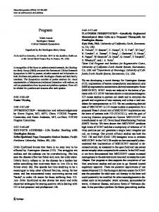
ADF TEST STATISTICBOOTSTRAP CORRECTED PROGRAM This program requires the input filename (without an extension that mnst be ".dat') that includes the raw data matrix of order n x p. Also it assumes that in the same directory there is a vector parameters file of order q x 1 with the same name but with "ipar" extension. At the end of the processthe program will create one output file with the same name and the ".out' extension. Please answer the followingquestions: Input data matrix file name: Number ofcases: Number ofvariables ofthe model: Number ofparameters to estimate:

EXAMPLE

1300 111 133

b..---------------------------=-----------::------COMPUTING THE ADF WEIGHT MATRIX W Skewness= 7.059 p= 0.003 Kurtosis= 142.716p= 0.558

c

MINIMIZING THE ADF DISCREPANCY FUNCTION Iteration: 1 ADF Function: 0.149724 Max Gradient: 0.005801

d

COMPUTING BOOTSTRAP W MATRIX Extracting 500 boot samples, it will take aprox, 30.00 seconds

e

MINIMIZING THE BOOTSTRAP ADFDISCREPANCY FUNCTION Iteration: 1 ADF_BOOT Function: 0.162341 Max. Gradient: 0.253501

f

OUTPUT T_adf = 44.917133 p= 0.080788 T_boot = 48.684004p= 0.038545 T_biasl = 41.150261 p= 0.155985 T_bias2 = 41.441719 p= 0.148710 Degrees offreedom = 33 5.225563 Mean error W_ad! - WJloot 0.004935 Mean error S_sample- S_boot Mean error Sigma_adf· Sigma_boot 0.‫סס‬OO70

Figure 1. (a) Input screen. (b) Screen display ofthe computation ofthe ADF matrix Wand the Mardia statistic. (c) Screen display ofthe process ofthe minimization ofthe ADP function. (d) Screen display ofthe 500 boot samples extraction process. (e) Screen display of the process of minimization of the ADF bootstrap function. (f) Screen display of the content ofthe output me.

HIGH-LEVEL LANGUAGE PROGRAM

299

Figure 2. Structural model of 11 observed variables, 5 factors, and 33 parameters to estimate.

FIT:

ERROR:

VALE:

FLEfS:

computation of the weight bootstrap matrix W~ (Equation 10). Returns the X 2 statistic likelihood and the standard error vector of parameters. Returns TADF;Bl and T A DF;B2 as well as their associated likelihood. Returns the average of the differences between the sample S matrix and the bootstrap average S~ matrix, as well as the difference between the ordinary I( y) and the I( y) generated from the minimization of the discrepancy function upon including S~ and W·. It finally computes the average of the differences between the ordinary weight matrix Wand the weight matrix W' generated from the bootstrap procedure. Procedure that, although not necessary for realization of the two corrections proposed by Yung and Bentler (1994), could be of great value in carrying out Monte Carlo simulations, generating random samples of size n in p variables, with skewness and kurtosis previously selected by the user, according to Vale and Maurelli (1983) algorithms. The Fleishman constants can be estimated using the following FLEfS procedure. Procedure that returns the Fleishman constants a, b, c, and d in order to get the expected skewness and kurtosis for a variable or set of variables.

The correct use of the program involves both the compilation of the ADF.G file (using the command COMPILE ADF.G), which includes the procedures, and the later call and execution of the ADF.GSS file (using the command RUN ADF.GSS), which contains the iterative procedure that accomplishes the required calls to the subroutines of the previous file. This execution produces the request for the

raw-data matrix filename, the number of cases, the variables, and the number of parameters to estimate (Figure la). The program assumes that, in the same directory, a vector with the starting values of the parameters exists with the same name as the data file, except that it has the extension ".par." This vector could be the ML or ADF solution of the commercially available packages. Obviously, the generation of the I(Yt) matrix from the BUILD procedure is exclusive to each model; for this reason, the user, before compiling the procedures file, must define the localization of all of the q parameters in order to estimate each of the structural model matrices (A, I", B, =

[ [9"+11 ,,,+12 9,,] '13 11 '3J 'J2

B33

B..

&33

e ....

l

B"

B..

,..

B11

'1'= IjIII IjI

IjI 12 ] 1jI"

l

Figure 3. Structural parameter matrices implemented in the BUILD procedure.

300

HERNANDEZ, RAMiREZ, AND SANCHEZ

Table 1 Rejection Rates of the Test Statistics in the Monte Carlo Simulation

Nonnormality Conditions n = 300

Statistic

Skew1.5-Kur3 SkewO-Kur6

n = 500 Skew3~Kurl5

Skew1.5-Kur3

SkewO-Kur6 Skew3-Kurl5

(X= .05 Ordinary .1355 .1137 .1060 .1125 .1166 .1082 Bootstrap .2135 .1970 .1469 .2066 .1633 .1365 B30r1 .0915 .0769 .0501 .0766 .0666 .0443 B cor2 .0983 .0903 .0537 .0833 .0666 .0443 Note-"Ordinary" is the ordinary ADF statistic; "Bootstrap" is the ADF test statistic from the B bootstrap samples; "B30rl" is the Bias, corrected ADF test statistic; and "B30r2" is the Bias, corrected ADF test statistic. "Skew" = skewness; "Kur" = kurtosis.

Table 2 Means and Standard Deviations ofthe Test Statistics in the Monte Carlo Simulation

Nonnormality Conditions

n = 300 SkewO-Kur6

n = 500 Skew3-Kurl5 Skew1.5-Kur3 SkewO-Kur6 Skew3-Kurl5 Statistic M SD M SD M SD M SD M SD M SD Ordinary 36.97 9.308 37.15 8.784 37.19 7.287 37.24 8.950 35.30 8.624 36.19 7.179 Bootstrap 39.64 10.08 39.58 9.851 39.55 8.332 39.70 9.964 37.81 9.596 38.55 8.092 B_cor1 34.29 9.375 34.71 8.620 34.83 7.245 34.78 8.766 32.78 8.413 33.83 7.206 B cor2 34.64 9.325 35.03 8.603 35.13 7.212 35.09 8.745 33.09 8.384 34.12 7.149 Note-"Ordinary" is the ordinary ADF statistic; "Bootstrap" is the ADF test statistic from the B bootstrap samples; "B30rl" is the Bias, corrected ADF test statistic; and "B30r2" is the Bias, corrected ADF test statistic. "Skew" = skewness; "Kur" = kurtosis. Skew1.5-Kur3

among 11 observed variables (Figure 2) (Joreskog & S6rborn, 1986). In this model, there are 33 parameters to estimate (33 df). The different matrices that will help the user to appropriately locate the 33 elements of the parameter vector are shown in Figure 3. To demonstrate the program's effectiveness and its corrective procedure, the ADF statistic found in our program for three different nonnormal data matrices was compared with the same statistics found in the LINCS program (Schoenberg & Arminger, 1988). Once the correct operation of the application was checked, a Monte Carlo simulation procedure was carried out using the model shown in Figure 2 and manipulating the sample size (300 and 500 cases) and nonnormality by observing variable skewness and kurtosis through three levels (Skew 0 - Kurt 6, Skew 1.5 - Kurt 3, Skew 3 - Kurt 15). For each one of the six 3 X 2 conditions, 300 independent samples were generated from the variance and covariance matrix in Joreskog and Sorborn (1986, p. III98) by means of the Fleishman (1978) and Vale and Maurelli (1983) algorithms, implemented in the VALE procedure. As shown in Table 1, irrespective of the sample size and of the skewness and kurtosis of the observed variables, the correct model rejection rates for the ordinary test statistic are higher than expected. In that same table, we can see that both corrections introduce acceptable rejection rates for kurtosis, in general not less than six, especially in the condition of skewness 3 and kurtosis 15, irrespective of the sample size. However, when the levels of kurtosis are less than that value, the bootstrap corrections do not particularly improve the results. Table 2

shows the empirical means and standard deviations of the investigated test statistic. As can be seen, the two bias corrections present values close to the expected 33 and 8.12. It is clear that the better outcome was obtained with 500 cases and a skewness of 3 and a kurtosis of 15. Discussion The execution of the program introduced is fast and efficient (see Table 3). It will not only permit the realization ofthe bootstrap correction proposed by Yung and Bentler (1994), but will also, as a result of the inclusion of the nonnormal random samples-generation procedure, facilitate the realization of Monte Carlo simulations in the newly proposed ADF test-statistic correction. Obviously, the Yung and Bentler (1994) correction needs further research with a wide variety of models as a function of the complexity of the same sample size, nonnormality, and so on, to confirm the effectiveness of the method in terms of a generalization of the results. On the other hand, given the nature of an open program of this type, it will facilitate the inclusion of new

Table 3 TIme of Execution of the Program for the Model Introduced in Terms of Sample Size

Sample Size 300 500 800 1,000 1,500 Elapsed time 0:47 1:15 1:55 2:21 3:22 Note-Time is given here in minutes:seconds. The computer was a Pentium at 90 MHz with 16MB of ram memory.

HIGH-LEVEL LANGUAGE PROGRAM procedures and improvements that will appear in the specialized literature and that undoubtedly will delay implementation in commercial programs. Also, it would be very simple to include other test statistics that are less computationally demanding, as it is with normal distribution test statistics. These tests could be maximum likelihood, generalized least square, as well as the elliptical distribution, since the Mardia-based multivariate kappa can be obtained very easily from the Mardia multivariate kurtosis statistic implemented in the MARDI procedure. For the inclusion of these methods, one simply needs to add the pertinent discrepancy functions, as well as a determination of the gradient and the hessian matrix that can be found in Browne (1984). Finally, when all the source codes are included, the program will permit great control and absolute manipulation ofall ofthe equations and variables, which could be very useful at a pedagogic level. Availability

The complete program described above can obtained from the first author (whose e-mail address is jhdez@ ull.es). REFERENCES APTECH SYSTEMS, INC. (1995). Gauss: The Gauss System Version 3.2. Washington: Author. BOLLEN, K. A. (1989). Structural equations with latent variables. New York: Wiley. BROWNE, M. W. (1974). Generalized least squares estimators in the analysis of covariance structures. South African Statistical Journal, 8,1-24. BROWNE, M. W. (1984). Asymptotically distribution-free methods for the analysis of covariance structures. British Journal ofMathematical & Statistical Psychology, 37, 62-83. BURDEN, R. L., & FAIRES, J. D. (1989). Numerical analysis (4th ed.). Boston: Prindle, Weber & Schmidt.

301

CHOU, c.-P., BENTLER, P. M., & SATORRA, A. (1991). Scaled test statistics and robust standard errors for non-normal data in covariance structure analysis: A Monte Carlo study. British Journal ofMathematical & Statistical Psychology, 44,347-357. CUDECK, R., & BROWNE, M. W. (1992). Constructing a covariance matrix that yields a specified minimizer and a specified minimum discrepancy function value. Psychometrika. 57, 357-369. CUDECK, R., KLEBE, K. J., & HENLY, S. 1. (1993). A simple GaussNewton procedure for covariance structure analysis with high-level computer languages. Psychometrika, 58, 211-232. FLEISHMAN, A. (1978). A method for simulating non-normal distributions. Psychometrika, 43, 521-531. HARLOW, L. L. (1985). Behavior of some elliptical theory estimators with non-normal data in a covariance structureframework: A Monte Carlo study. Unpublished doctoral dissertation, University of California, Los Angeles. Hu, L.- T., BENTLER, P. M., & KANO, Y. (1992). Can test statistics in covariance structure analysis be trusted? Psychological Bulletin, 112, 351-362. JORESKOG, K. G. (1969). A general approach 10 confirmatory maximum likelihood factor analysis. Psychometrika, 34, 183-202. JORESKOG, K. G., & SORBOM, D. (1986). LISREL VI: Analysis oflinear structural relationships by maximum likelihood and least squares methods. Mooresville, IN: Scientific Software, Inc. MARDIA, K. (1970). Measures of multivariate skewness and kurtosis with applications. Biometrika, 57, 519-530. MARDIA, K. (1974). Application of some measures of multivariate skewness and kurtosis in testing normality and robustness studies. Sankhya: The Indian Journal ofStatistics, 36, 115-128. MUTHEN, B., & KAPLAN, D. (1992). A comparison of some methodologies forthe factor analysis ofnon-normal Likert variables: A note on the size ofthe model. British Journal ofMathematical & Statistical Psychology, 45, 19-30. SCHOENBERG, R., & ARMINGER, G. (1988), LlNCS2: A program for linear covariance structure analysis. Kensington, MD: RJS Software. VALE, D., & MAURELLI, V. A. (1983). Simulating multivariate nonnormal distributions. Psychometrika, 48, 465-471. YUNG, Y.-F., & BENTLER, P. M. (1994). Bootstrap-corrected ADF test statistics in covariance structure analysis. British Journal ofMathematical & Statistical Psychology, 47, 63-84. (Manuscript received June 29, 1995; revision accepted for publication December II, 1995.)