A high-resolution frequency variable experimental setup for studying ferrofluids used in magnetic hyperthermia E. E. Mazon, E. Villa-Martínez, A. Hernández-Sámano, T. Córdova-Fraga, J. J. Ibarra-Sánchez, H. A. Calleja, J. A. Leyva Cruz, A. Barrera, J. C. Estrada, J. A. Paz, L. H. Quintero, and M. E. Cano
Citation: Review of Scientific Instruments 88, 084705 (2017); doi: 10.1063/1.4998975 View online: http://dx.doi.org/10.1063/1.4998975 View Table of Contents: http://aip.scitation.org/toc/rsi/88/8 Published by the American Institute of Physics
Articles you may be interested in A multi-frequency electrical impedance tomography system for real-time 2D and 3D imaging Review of Scientific Instruments 88, 085110 (2017); 10.1063/1.4999359
REVIEW OF SCIENTIFIC INSTRUMENTS 88, 084705 (2017)
A high-resolution frequency variable experimental setup for studying ferrofluids used in magnetic hyperthermia 1 T. Cordova-Fraga, 2 ´ ´ ´ E. E. Mazon,1 E. Villa-Mart´ınez,2 A. Hernandez-S amano, 3 4 1,5 1 ´ J. J. Ibarra-Sanchez, H. A. Calleja, J. A. Leyva Cruz, A. Barrera, J. C. Estrada,1 J. A. Paz,1 L. H. Quintero,1 and M. E. Cano1,a)
1 Centro Universitario de la Ci´ enega, Universidad de Guadalajara, Av. Universidad 1115, Col. Linda Vista, Ocotl´an, Jalisco C.P. 47820, Mexico 2 Departamento de F´ısica, Divisi´ on de Ciencias e Ingenier´ıas Campus Le´on, Universidad de Guanajuato, Loma de Bosque 103, Col. Lomas del Campestre, C.P. 37150 Guanajuato, Mexico 3 Departamento de Ingenier´ıa Qu´ımica, Divisi´ on de Ciencias Naturales y Exactas, Campus Guanajuato, Universidad de Guanajuato, Noria Alta S/N, Noria Alta, 36050 Guanajuato, Gto., Mexico 4 Centro Nacional de Investigaci´ on y Desarrollo Tecnol´ogico, Interior Internado Palmira S/N, Palmira, 62490 Cuernavaca, Mor., Mexico 5 Universidade Estadual de Feira de Santana, Av. Transnordestina, s/n, Novo Horizonte, 44036-900 Feira de Santana, BA, Brazil
(Received 17 October 2016; accepted 31 July 2017; published online 24 August 2017) A scanning system for specific absorption rate of ferrofluids with superparamagnetic nanoparticles is presented in this study. The system contains an induction heating device designed and built with a resonant inverter in order to generate magnetic field amplitudes up to 38 mT, over the frequency band 180-525 kHz. Its resonant circuit involves a variable capacitor with 1 nF of capacitance steps to easily select the desired frequency, reaching from 0.3 kHz/nF up to 5 kHz/nF of resolution. The device performance is characterized in order to compare with the theoretical predictions of frequency and amplitude, showing a good agreement with the resonant inverters theory. Additionally, the setup is tested using a synthetic iron oxide with 10 ± 1 nm diameter suspended in liquid glycerol, with concentrations at 1%. Meanwhile, the temperature rise is measured to determine the specific absorption rate and calculate the dissipated power density for each f. This device is a suitable alternative to studying ferrofluids and analyzes the dependence of the power absorption density with the magnetic field intensity and frequency. Published by AIP Publishing. [http://dx.doi.org/10.1063/1.4998975]
I. INTRODUCTION
Recently, the study and development of magnetic nanoparticles (MNPs) for biomedical applications in thermotherapy have substantially increased. In the magnetic hyperthermia area, new iron oxide materials are being synthesized with low polydispersity in diameters and strong magnetic properties, using more controlled synthesis methods.1–4 As the heating of MNPs exhibits a strong dependence between the applied magnetic field intensity H of frequency f and their diameters σ, it is always desirable to reach good homogeneity of the MNP sizes to achieve the best heating control. In a hyperthermia experiment, it is important to appropriately select f and H depending on the magnetic susceptibility, χMP , and anisotropy constant, κ, of the MNPs, in order to reach high heating but using a low concentration of MNPs. The physical magnitude that indicates the warming capability of MNPs through an alternating magnetic field is the specific absorption rate (SAR). Indeed, the biocompatible and noninteracting superparamagnetic iron oxide nanoparticles (SPIONs) are an attractive choice in the labeling of carcinogenic cells for in vivo experiments,5 with diameters from 5 to 20 nm.5–7 a)
Authors to whom correspondence should be addressed: eduardo.cano@ cuci.udg.mx and
[email protected]
0034-6748/2017/88(8)/084705/7/$30.00
Commonly, the warming of SPIONs with high-frequency magnetic fields is generated using induction heating devices, employing radiofrequency amplifiers,8–12 or developing resonant inverter systems.13–18 Nevertheless, both alternatives need a resonant circuit. The first devices imply high costs because they involve commercial amplifier apparatus designed for industrial applications and with output impedance 50 Ω. Hence, the supplied current to the resonant-circuit could be limited. In contrast, the resonant inverter systems include a switching circuit (called inverter) of semiconductors to feed a resonant circuit, and following an initial design, it is possible to achieve a more controlled magnetic field generator on a frequency band. Typically, these inverter circuits could be selected as H-bridge, push-pull, or chopper interrupters.19 The resonant circuits are composed of inductive plus capacitive elements, which are connected either in parallel or series configurations and more complex configurations including combinations of them.20 Furthermore, the induction heating devices are complemented with Fluoroptic thermometers to measure the SAR of ferrofluids.8–18 Some of these heaters are designed to work with a fixed frequency,13–15,21 but it can be modified replacing the work inductor. This procedure could be tedious and impractical. Meanwhile, other induction heaters with adjustable frequency are complemented with AC magnetometers to measure the complex susceptibility, which is
88, 084705-1
Published by AIP Publishing.
084705-2
Mazon et al.
Rev. Sci. Instrum. 88, 084705 (2017)
directly related with the nanoparticles SAR. Even the inverters are designed to select f in an established range; in some cases, this range is insufficient 12,23 while others are limited in frequency resolution11,12,22 or H magnitude.22 Indeed, the main aim of this work is to design and construct an experimental setup to study the dependence of the power density absorbed for a ferrofluid with the frequency and amplitude of the applied magnetic field. In contrast to other studies, the designed system can easily select up to 300 resonant frequencies because the user only sets the corresponding capacitance with the desired frequency. Thus, this represents a new reliable, powerful, and versatile alternative.
predict the tissue heating. An indirect way is through the SAR determination of the ferrofluid with total density, ρF , following the equation26 P = ρF ∗ SAR. (2) In Eq. (3), SAR is defined as a function of the specific heat C v (at low concentrations of SPIONs, it is approximated just to the specific heat of the liquid medium), fraction of nanoparticles mnp , and temperature rise over time dT /dt, SAR =
Cv dT . mmp dt
(3)
B. Resonant inverter systems II. THEORETICAL BACKGROUND A. Heating magnetic nanoparticles
When a ferrofluid of SPIONs is submitted to an AC magnetic field H, it dissipates energy depending on its magnetic susceptibility χF and magnetic relaxation time τ, called the N´eel-Brown relaxation time. As was stated by Rosensweig, the dissipated power density P in the ferrofluid volume satisfies Eq. (1),24 which sometimes is known as an approximation of the linear response theory (LRT). Nevertheless, recently Carrey et al.25 have stated that the ferrofluid heating always obeys a hysteresis loop, independently of their nanoparticle sizes. So, the dynamic determination of P is also recommendable. However, the constriction µ0 M s VH < k B T is a valid criterion to ensure the correct approximation of Eq. (1) using low field, superparamagnetic nanoparticles of volume V and saturation magnetization M s ,24 P = 2.48 × 10⁻⁵ χF H 2 f 2
τ 1 + (2πf τ)2
.
(1)
The characterization of ferrofluids through its P value is important for studies of magnetic hyperthermia in order to
The inverter circuits made with a half H-bridge possess good stability for switching currents, and its activation control is easier than the inverters with full H-bridge configuration,27 which are designed to feed electric loads with high power consumption. In either case, for applications in the range of 1 kHz–1 MHz, the metal-oxide semiconductor field-effect transistor (MOSFET) technology is widely recommended. In the theory of LC circuits, it is known that their resonance conditions depend on the specific topology implemented. For instance, ideally, LC series circuit manifests null total impedance Z T and a voltage gain when the resonance condition (unique) is satisfied, while the LC parallel circuit offers a current gain and infinite Z T . Moreover, all those properties can be exploited in mixed and more complex network topologies.20 Figure 1(a) displays the LC-LC resonant circuit and its equivalent circuit is shown in Fig. 1(b), which contains an L S C S series circuit with the inductance L S and static capacitance C S . This circuit is connected to an L P C P parallel circuit, which contains a variable C P capacitor displayed in Fig. 1(c). L S C S provides short circuit immunity to the inverter device and adequate voltage gain to feed L P C P . With this tension, we can generate a high resonant current in the solenoid
FIG. 1. Diagrams of (a) the control stages including the power inverter and the LC-LC resonant circuit, (b) its equivalent circuit, and (c) the rotary variable capacitor diagram Cp.
084705-3
Mazon et al.
Rev. Sci. Instrum. 88, 084705 (2017)
FIG. 2. The electric current dependence with frequency, which is flowing through the coils Ls (dark rectangles) and Lp (solid line), exhibiting two series-resonances (I LS maximum) and one parallel resonance (minimum I LS ).
L P to produce the desired magnetic field H and heat magnetic materials. To know the resonant behavior of this L S C S –L P C P ideal circuit, the AC Ohm law is used as shown in Eq. (4). Considering its total reactance for any angular frequency ω and applying the series resonance condition (Z T = 0) for ω0 , also with A = (C s L s C p L p ) and B = (C s L s + C p L p + C s L p ), Eq. (4) is reduced to the biquadratic equation (5). Only two positive solutions expressed by Eqs. (6) and (7) have physical sense. Meanwhile, the unique possibility of obtaining an infinite Z T is given by Eq. (8), ZT = ωLs −
ωLp 1 + = 0, ωCs 1 − ω2 Cp Lp
Aω4 − Bω2 + 1 = 0, q √ B + B2 − 4A 1 ω0 = , √ 2A q √ B − B2 − 4A ω03 = , √ 2A ωp = p
1 . Lp Cp
(4) (5) (6)
III. MATERIALS AND METHODS
The magnetic scanning system comprises a set of electronic apparatus, which are specifically assembled to determine the SAR [through Eq. (3)] of ferrofluids with specific heat C v , and the device is suitable to adjust the values H and f. In Fig. 3, the resonant inverter (A) is observed, which is powered by a DC power supplier Xantrex XFR150-8 (B). Also, a function generator (C) provides a rectangular signal with frequency f and amplitude 10 V to drive the inverter. The resonant circuit includes a cylindrical coil L p (D) to generate H through a resonant current. This value is measured with a current probe Tektronix A6303 (E) using its corresponding amplifier AM503 (F) connected to the oscilloscope (G). As the ferrofluid is placed inside the coil cavity, a Fluoroptic thermometer Luxtron-One (H) is employed to measure its temperature rise. These readings are stored in a laptop (I), working in the LabView environment. Additionally, the resonant inverter
(7) (8)
To exemplify the operation of the L S C S –L P C P circuit, two curves obtained from P-SPICE are displayed in Fig. 2, and the following values are considered: L s = 8.2 µH, L p = 3.8 µH, C s = 200 nF, C p = 37 nF, even including equivalent resistances RLS = 2.98 Ω and RLP = 0.01 Ω of the inductors L s and L p , respectively. The dark rectangles represent the current flowing through L s in a frequency range 50–520 kHz, exhibiting two maximum values corresponding to ω01 and ω03 of Eqs. (6) and (7), plus the minimum value ωP associated with the infinite Z T condition applied in Eq. (8). Furthermore, analyzing the current flowing through L p (solid line), a major peak is clearly observed at ω01 . Accordingly, the C p values of the variable capacitor described in Fig. 1(c) must be chosen to maintain the constant working of the resonant inverter in this regimen.
FIG. 3. Full experimental setup showing the resonant inverter (A) powered with the DC power supply (B) and also connected with the function generator (C); the current probe (E) with its amplifier (F) connected to an oscilloscope (G); and the optic-thermometer (H) coupled to a PC (I) to measure the temperature.
084705-4
Mazon et al.
is cooled with a water flux of 3 l/min as the components of these circuits are sensitive to temperature, which can decrease their efficiency and even could be destroyed. In the same sense, in Fig. 4(a), a close-up of a transversal view of L p is shown. This coil is winded in total with N = 20 loops of the isolated copper tube over two layers (ten per layer); the total length is l = 5 cm with an inner diameter of 2.5 cm. Thereby, in this cavity, the sample holder is placed with ferrofluid inside, which is in contact with an optical fiber sensor and there is an isolating medium (glass wool) between L p and the sample holder. In Fig. 4(b), an exploded perspective view of all the pieces to be placed inside L p is shown. A cylindrical cavity is observed in the holder cap that can secure the fiber, keeping it in a constant position. This procedure is followed as described by Wang et al.29,30 For its part, the resonant inverter device of Figs. 4(a) and 4(b) is built using the diagram of Fig. 1(a) and considering the following values: L s = 8.64 µH, L p = 3.8 µH, C s /2 = 100 nF [the half value of C s in Fig. 1(b)], and C p = 37–337 nF. L s is built with litz wire to diminish its skin effect, and all the capacitors are manufactured with polypropylene. Indeed, the variable capacitor C p was performed modifying a decade capacitor using a fixed capacitance C fixed = 37 nF to which capacitors in parallel can be connected to increase the equivalent capacitance with a resolution of 1 nF reaching up to 337 nF. Additionally, each capacitor is activated via rotary switches using the scheme of C p displayed in Fig. 1(c). This chosen L S C S – L P C P circuit represents an improvement of the one used in our previous paper,13 which was constructed with a full H-bridge and could work with only fixed frequency. As can be observed in Fig. 1(a), in this new design, we have only a half H-bridge, which includes two capacitors (Cs/2 = 100 nF) replacing two switching transistors of the previous full-bridge design [see Fig. 1(b) of Ref. 13]. Additionally the new parallel capacitor C p is variable. Nevertheless, both electronic topologies have the same draining power capability and sinusoidal waveform. Indeed, the resonant circuit of Fig. 1(b) is equivalent to the one in Fig. 1(a).28 When a switch is activated, both capacitors
Rev. Sci. Instrum. 88, 084705 (2017)
C s /2 work in parallel, doubling the resonant current. Moreover, the used driver for the activation of the transistors Q1 and Q2 (technology IXNK75N60C) is simpler than that in the previous studies.13,15 This is composed for a pair of complementary MOSFET-drivers IXDN614CI and IXDI614CI, which at their inputs acquire the rectangular signal of the function generator (duty cycle 40%) to be pre-amplified. Their outputs signals are shifted 180◦ and each one feeds a toroidal transformer (as galvanic isolation) to be connected to the gate terminals of Q1 and Q2. Antiparallel diodes are also used to suppress counterelectromotive forces and snubber circuits with charging time 1 µs. Posterior to the computer simulation of the resonant inverter, electronic work, and assembling, the full setup is tested to experimentally determine each ω01 feeding with 1 A. This procedure is carried out by manually tuning the function generator to the frequencies where the maximum values of the resonant current I LP crossing L p for each selected C p were obtained. In another vein, magnetic uncoated nanoparticles of magnetite with σ = 10 ± 1 nm diameter, density ρ = 5180 kg/m3 , and initial magnetic susceptibility χmp = 1.823 ± 0.325 (MKS) are synthesized by thermal decomposition in our chemistry lab.31 This value of χmp was corroborated using a VSM lakeshore 7300. Thus, the magnetic susceptibility of the ferrofluid is given by Eq. (9), where the diamagnetic susceptibility of glycerol χGly = 9.82 × 10 6 , χF = mmp χmp + nGly χGly .
(9)
To start our experimental setup with ferrofluids, three identical samples with 1 ml of ferrofluid in sample-holders have been prepared (called M1, M2, and M3) using mmp = 1% of magnetite suspended in nGly = 99% of pure glycerol to diminish its sedimentation time. Thus, we have χF = 0.018 22 ± 0.003 25. In addition, another sample holder with 100% of glycerol as a “negative sample” is used. On the other hand, in order to obtain the ferrofluid SAR using Eq. (3), with mmp = 0.01 and C v = 2382.7 J/kg K, only the
FIG. 4. (a) Close-up of a transversal view of the resonant coil with the holder inside, containing ferrofluid making contact with the optical fiber sensor. (b) Exploded perspective view of all the pieces placed inside the coil cavity.
084705-5
Mazon et al.
Rev. Sci. Instrum. 88, 084705 (2017)
heating rate (dT /dt) needs to be determined. The procedure starts by placing the ferrofluid in contact with the temperature sensor within the adiabatic cavity, and this lasts inside the resonant coil L p as detailed in Figs. 4(a) and 4(b). Posteriorly, f is selected in the function generator, and then the corresponding C p is tuned to generate H, whose magnitude is chosen from the power supply. Thus, the ferrofluid is irradiated over 2 min to be heated. Since the adiabatic mean is not ideal, the slope dT /dt of the negative sample is quantified in the first step. Later the slope dT /dt of each ferrofluid sample is measured (immediately after being stirred), and the mean value hdT /dti is computed, including its standard deviation. Once again, the negative sample is analyzed to verify the non-variation of the background heating rate. Finally, the value dT /dt of the negative sample (almost always approximately 0.004 K/s) is subtracted from hdT /dti to obtain the ferrofluid SAR. Thereby, using Eq. (2) and ρF = 1250 kg/m3 , we have just a point of the dissipated power density plot P vs. f. IV. RESULTS AND DISCUSSIONS
In a first test of the device operation and working without sample inside of L P , a frequency of 523 kHz is selected; the rectangular pulse provided by the function generator is obtained from the oscilloscope and shown at the top of Fig. 5(a). The output signals of the MOSFET drivers are also displayed at the bottom of Fig. 5(a). Both signals are used to activate the gate terminals through a toroidal transformer, and they are clearly shifted 180◦ with a duty cycle of 40%. Meanwhile, the resonant current I LP crossing L P is measured with the current probe and another oscilloscope. At the top of Fig. 5(b), the sinusoidal dependence is observed, while in the bottom of the figure, the FFT is computed to evidence the absence of harmonic components in I LP . Hence, in Fig. 6, the C p values in the range 37–337 nF are correlated with each resultant frequency ranging from 180 to ω1
525 kHz. The dark symbols are the values of f = 2π0 calculated with Eq. (6), and the experimental resonant frequencies are the
FIG. 6. Plot Cp vs f theoretical (dark symbols) and experimental (empty symbols) frequencies.
open squares, showing maximum discrepancies of up to 1% for the highest values of C p . The programmed capacitances from 337 nF to 237 nF are swept following 10 nF steps of capacitances, reaching 3 kHz of frequency steps approximately with an almost linear dependence on the capacitance. Thus, 0.3 kHz/nF is the obtained resolution. In the interval from 237 nF to 137 nF, 5 nF steps of capacitance are used, allowing 2 kHz steps of frequency approximately. Also in this range, the linear dependence shows a qualitative agreement, then 0.4 kHz/nF is the approximated resolution. The last interval from 137 nF to 37 nF was swept with 2 nF steps of capacitance; nevertheless, a linear dependence shows a bad approximation in this range as the resolution varies from 1.5 kHz/nF to 5 kHz/nF. The three intervals together, provide us up to 300 possible tuning frequencies, representing a versatile option for ferrofluid analysis or magnetic hyperthermia applications. In contrast with other setups, which are designed to work with fixed frequencies,13–15,21 where the coil Lp must be replaced to modify the desired frequency. Moreover, in order to improve the tuning resolution 5 kHz/nF for high frequencies, at least another decade stage of capacitance could be added to C p , reducing the steps of capacitance.
FIG. 5. (a) Rectangular signal (top) provided for the function generator with f = 523 kHz and the output signals of the MOSFET drivers shifted 180◦ (bottom); (b) the sinusoidal resonant current with its computed FFT.
084705-6
Mazon et al.
FIG. 7. Theoretical (dark sphere) and experimental (open rhombus) output current crossing the resonant coil L P and feeding the whole setup with 4 ARMS .
Following the characterization of the resonant inverter, the values of I LP are measured over the frequency range 180–525 kHz, keeping a constant input current I 0 = 4 ARMS and assuming an equivalent total resistance RE = 2.92 Ω. As observed in Fig. 7, the experimental curve (open rhombus with error bar) shows an increment up to a maximum value at 263 kHz, followed by a decreasing trend, which reaches a relative minimum value, to continue again with an almost plane trend. In fact, the ideal theoretical values (dark spheres) exhibit a good agreement with the experimental measurements with a maximum discrepancy 10% at 275 kHz, which can be related to power switching losses. Using the definition of current gain G of the circuit through the formula G = IILP0 , the maximum gain ¯ = 7.13 ± 1.12 are observed. An GMAX = 8.25 and mean gain G alternative for obtaining constant ILP over the full frequency range could be carried out by introducing a control function of the input current. Indeed, the used power supply Xantrex
Rev. Sci. Instrum. 88, 084705 (2017)
XFR150-8 already possesses digital and analogical input terminals, which can be used to modulate the input current supplied to the inverter circuit. With the value I LP , the amplitude of the sinusoidal magnetic field intensity is estimated by H = ILPl N . For example, when the current value (RMS) is I LP = 28.5 A, it allows a peak amplitude H = 16 kA/m, feeding the entire system with 4 ARMS . In this setup, the maximum H recommendable is 30 kA/m to avoid an over-current to the switching transistors. In relation to the SAR determination, a typical graph T vs. t measured with this experimental setup is shown Fig. 8(a) by applying f = 492 kHz and H = 20 kA/m to warm each ferrofluid sample (M1, M2, and M3). Also, two measurements of the negative sample are plotted before and after the warming of ferrofluids (named control 1 and control 2, respectively). With a fast observation of all the curve slopes, the differences between the heating rates of ferrofluids (major slope) and the negative sample (minor slopes) are evidenced. Now, hdT /dti can be calculated to obtain the corresponding P value via Eq. (2). In the same sense, Fig. 8(b) shows twenty measurements of P (dark spheres) in the range 180–525 kHz with this H value. Meanwhile, using the obtained validity criterion of Eq. (1), i.e., 3.42 × 10 21 J < 4.14 × 10 21 J, a data regression is carried out and represented by the continuous line in the same figure. To analyze the regression quality, the parameter X2 by Eq. (10) is calculated, where n = 20 is the number of measurements and g = 2 is the number of parameters to be determined. Also for each i-value, Pi and P(x i ) represent the theoretical and measured dissipated power densities with the estimated error S i , X2 =
1 X (P(xi ) − Pi )2 . i n−g Si2
(10)
Thus, the estimated magnitudes are χF = 0.0137 ± 0.0005 and τ = 6.8 ± 0.6 × 10 7 s that satisfies X2 = 0.985, indicating a good fit. In accordance with Taylor,32 the higher quality of
FIG. 8. (a) Typical measurements of the temperature rise of the three ferrofluid samples plus the measurements of the negative sample, using f = 492 kHz and H = 20 kA/m; (b) the dissipated power density in the range of 180–525 kHz (dark spheres) adding the regression fit (solid line) using Eq. (1).
084705-7
Mazon et al.
Rev. Sci. Instrum. 88, 084705 (2017)
ACKNOWLEDGMENTS
Authors wish to thank the Mexican institution CONACYT for the scholarship of the undergraduate and graduate students and also thank Thomas Trent for reviewing the language of the paper. 1 J.
FIG. 9. Measurements of P (dark spheres) with f = 492 kHz considering six different values of H and the plot of theoretical Eq. (1) (solid line).
the regression is reached when X2 = 1. Indeed, the magnetic susceptibility of the ferrofluid is 25% lower that of the real value. Once the magnitudes χF and τ of Eq. (1) for this ferrofluid are encountered, the experimental setup is employed to determine P, but on changing the experimental conditions, f = 492 kHz is fixed and H is gradually increased. Six experiments were carried out with the aim to compare the results of Eq. (3) with the corresponding theoretical prediction through Eq. (1) (using the fitted values χF = 0.0137 ± 0.0005 and τ = 6.8 ± 0.6 × 10 7 ). The measurements and error bars (dark spheres) are plotted in Fig. 9, where the solid line represents the theoretical curve. Further analysis is performed using Eq. (10), reaching X2 = 0.995, indicating a good fit quality. V. CONCLUSIONS
In this work, a multifrequency system to study ferrofluids was carried out. In contrast with other experimental setups, the device includes a versatile alternative to select the desired frequency over the interval 180–525 kHz, with 5 kHz/nF of minimum resolution for lower capacitances. Also for higher capacitances, 0.3 kHz/nF is the minimum reached resolution. In addition, its performance exhibits a good agreement with the theoretical frequency predictions, generates maximum magnetic intensities of 30 kA/m, and reaches a mean current gain G = 7.13 ± 1.12 in the resonant coil. Also, the whole system is suitable to determine the power absorbed density P of a ferrofluid with low nanoparticle concentrations and to analyze its dependence of P vs. f or P vs. H. Indeed, with these curves, it is possible to infer an approximated value of other important parameters of the ferrofluid [provided that Eq. (1) is valid] such as the equivalent magnetic susceptibility and the effective relaxation time.
Park, E. Lee, N. M. Hwang, M. Kang, S. C. Kim, Y. Hwang, J. G. Park, H. J. Noh, J. Y. Kim, J. H. Park, and T. Hyeon, Angew. Chem. 117(19), 2932 (2005). 2 T. Hyeon, Chem. Commun. 8, 927 (2003). 3 N. R. Jana, Y. Chen, and X. Peng, Chem. Mater. 16(20), 3931 (2004). 4 S. Sun and H. Zeng, J. Am. Chem. Soc. 124(28), 8204 (2002). 5 W. Lin, Y. W. Huang, X. D. Zhou, and Y. Ma, Toxicol. Appl. Pharmacol. 217(3), 252 (2006). 6 A. K. Gupta and M. Gupta, Biomaterials 26(18), 3995 (2005). 7 U. Schwertmann and R. M. Cornell, Iron Oxides in the Laboratory: Preparation and Characterization (John Wiley & Sons, New York, 2008), p. 183. 8 G. Vallejo-Fernandez, O. Whear, A. G. Roca, S. Hussain, J. Timmis, V. Patel, and K. O’Grady, J. Phys. D: Appl. Phys. 46(31), 312001 (2013). 9 O. Kaman, P. Veverka, Z. Jir´ ak, M. Maryˇsko, K. Kn´ızˇ ek, M. Veverka, ˇ P. Kaˇspar, M. Burian, V. Sepel´ ak, and E. Pollert, J. Nanopart. Res. 13(3), 1237 (2011). 10 E. Kita, H. Yanagihara, S. Hashimoto, K. Yamada, T. Oda, M. Kishimoto, and A. Tasaki, IEEE Trans. Magn. 44(11), 4452 (2008). 11 E. Garaio, J. M. Collantes, F. Plazaola, J. A. Garcia, and I. CastellanosRubio, Meas. Sci. Technol. 25(11), 115702 (2014). 12 L. M. Lacroix, J. Carrey, and M. Respaud, Rev. Sci. Instrum. 79(9), 093909 (2008). 13 M. E. Cano, A. Barrera, J. C. Estrada, A. Hernandez, and T. Cordova, Rev. Sci. Instrum. 82(11), 114904 (2011). 14 C. C. Tai and C. C. Chen, PIERS Online 4(2), 276 (2008). 15 M. E. Cano, T. C´ ordova, A. Hern´andez, J.C. Estrada, P. Knauth, Z. L´opez, M. Sabanero, and M. Sosa, Rev. Mex. Fis. S 58(2), 262 (2012). 16 C. C. Tai and M. K. Cheng, PIERS Online 4(4), 417 (2008). 17 S. W. Chen, J. J. Lai, C. L. Chiang, and C. L. Chen, Rev. Sci. Instrum. 83(6), 064701 (2012). 18 Z. Wu, Z. Zhuo, D. Cai, J. A. Wu, J. Wang, and J. Tang, Technol. Health Care 23(s2), S203 (2015). 19 B. D. Bedford and R. G. Hoft, Principles of Inverter Circuits (John Wiley & Sons, New York, 1964), p. 413. 20 S. Dieckerhoff, M. J. Ruan, and R. W. De Doncker, in IEEE Industry Applications Conference, Thirty-Fourth IAS Annual Meeting Conference Record (IEEE, 1999), Vol. 3, pp. 2039–2045. 21 M. Bekovi´ c, M. Trlep, M. Jesenik, V. Gorican, and A. Hamler, J. Magn. Magn. Mater. 355, 12 (2014). 22 M. Bekovi´ c and A. Hamler, IEEE Trans. Magn. 46, 552 (2010). 23 V. Connord, B. Mehdaoui, R. P. Tan, J. Carrey, and M. Respaud, Rev. Sci. Instrum. 85, 093904 (2014). 24 R. E. Rosensweig, J. Magn. Magn. Mater. 252, 370 (2002). 25 J. Carrey, B. Mehdaoui, and M. Respaud, J. Appl. Phys. 109(8), 083921 (2011). 26 D. W. Armitage, H. H. LeVeen, and R. Pethig, Phys. Med. Biol. 28(1), 31 (1983). 27 J. Feng, Y. Hu, W. Chen, and W. Chau-Chun, “ZVS analysis of asymmetrical half-bridge converter,” in IEEE 32nd Annual Power Electronics Specialists Conference (IEEE, 2001), Vol. 1, pp. 243–247. 28 M. K. Kazimierczuk and D. Czarkowski, Resonant Power Converters (John Wiley & Sons, New York, 2011), p. 154. 29 S. Y. Wang, S. Huang, and D. A. Borca-Tasciuc, IEEE Trans. Magn. 49(1), 255 (2013). 30 S. Huang, S. Y. Wang, A. Gupta, D. A. Borca-Tasciuc, and S. J. Salon, Meas. Sci. Technol. 23(3), 035701 (2012). 31 J. J. Ibarra-S´ anchez, R. Fuentes-Ram´ırez, A. G. Roca, M. del Puerto Morales, and L. I. Cabrera-Lara, Ind. Eng. Chem. Res. 52(50), 17841 (2013). 32 J. Taylor, Introduction to Error Analysis: The Study of Uncertainties in Physical Measurements (University Science Books, New York, 1982), p. 158.