Those reductions of the field degree increase efficiency in the SQRT implementation. More specifically the Tonelli-Shanks algorithm and the proposed algorithm ...
A High-Speed Square Root Algorithm in Extension Fields Feng Wang, Yasuyuki Nogami, and Yoshitaka Morikawa Dept. of Communication Network Engineering, Okayama University, Okayama-shi, 700-8530, Japan {wangfeng, nogami, morikawa}@trans.cne.okayama-u.ac.jp
Abstract. A square root (SQRT) algorithm in GF (pm ) (m = r0 r1 · · · rn−1 2d , ri : odd prime, d > 0: integer) is proposed in this paper. First, the Tonellid Shanks algorithm is modified to compute the inverse SQRT in GF (p2 ), where most of the computations are performed in the corresponding subi fields GF (p2 ) for 0 i d − 1. Then the Frobenius mappings with an addition chain are adopted for the proposed SQRT algorithm, in which a lot of computations in a given extension field GF (pm ) are also reduce to those in a proper subfield by the norm computations. Those reductions of the field degree increase efficiency in the SQRT implementation. More specifically the Tonelli-Shanks algorithm and the proposed algorithm in GF (p22 ), GF (p44 ) and GF (p88 ) were implemented on a Pentium4 (2.6 GHz) computer using the C++ programming language. The computer simulations showed that, on average, the proposed algorithm accelerates the SQRT computation by 25 times in GF (p22 ), by 45 times in GF (p44 ), and by 70 times in GF (p88 ), compared to the Tonelli-Shanks algorithm, which is supported by the evaluation of the number of computations.
1
Introduction
The task of computing square roots (SQRTs) in a finite field GF (pm ) is a problem of considerable importance. Why is the SQRT important? Of course, we may simply be interested in the problem because it’s there, but there are also applications to cryptography [1], [2]. In this paper, an efficient algorithm is proposed to compute the SQRT in GF (pm ). First, however, we give a short overview of several SQRT algorithms in a prime field GF (p). In order to find the values of z in z 2 = x for a given square x ∈ GF (p), most of known efficient methods are equivalent to or use the same basic ideas as either the Tonelli-Shanks [3] or the Cipolla-Lehmer algorithm [4]. The Cipolla-Lehmer algorithm has the disadvantage that one has to require a quadratic non-residue (QNR) that depends on both p and x, while the QNR needed by the TonelliShanks algorithm can be reused for different x. This study is based on the Tonelli-Shanks algorithm. The Tonelli-Shanks algorithm was originally devised in GF (p), but can easily be applied in GF (pm ) by simply replacing the operations in GF (p) with those in
GF (pm ). Note that the operations in GF (pm ) are more expensive than those in GF (p) for m > 1. For example, a multiplication in GF (pm ) at least requires m2 multiplications in GF (p) by using the schoolbook method. Therefore, it costs too much to directly apply the Tonelli-Shanks algorithm in extension fields. This is a big motivation of the authors to develop an efficient SQRT algorithm in extension fields GF (pm ). An extension field GF (pm ) provides us flexibility to choose system parameters, such as characteristic p and extension degree m as well as modular polynomial. The authors have considered the cases of m = 2d [5] and m = r2d [6], where r is an odd number and d � 0 is an integer. However, for the application to elliptic curve cryptosystem, we especially restricted d = 1, 2 in [6]. In this paper, we treat the general case i.e. p is an odd prime number and m has the form of m = r0 r1 · · · rn−1 2d , where ri is an odd prime number, and ri � rj for i � j, and d � 0 is an integer. In what follows m = r2d (r = r0 r1 · · · rn−1 ) without further explanation. The basic idea of the proposed SQRT algorithm is described as follows. If a given element x ∈ GF (pm ) is not a quadratic residue (QR), i.e. x has no SQRT in the same field, then there is no need to compute its SQRTs. Before SQRT m computations, we should thus use Euler’s criterion C m (x) = x(p −1)/2 to identify whether x is a QR or not, which is called QR test. Since m = r2d , the exponent in Euler’s criterion can be factorized into d d p2 − 1 pm − 1 =e· , e = 1 + p2 + · · · + (p2 )r−1 . 2 2 d
(1.1)
So, C m (x) can be evaluated in the following steps: 2d
C m (x) = x ¯(p
−1)/2
, x ¯ = N2md (x) = xe ,
(1.2)
where N2md (x), the norm of x with respect to the subfield GF (p2 ), is always an d element in GF (p2 ). From Eq.(1.2), i.e. x ¯ = xe , we have √ 1 x = x(e+1)/2 x ¯− 2 . (1.3) d
Based on Eq.(1.3), an efficient SQRT algorithm can be presented. In the proposed algorithm, the SQRT algorithm presented in [5], i.e. the MW-ST al1 gorithm, is first modified to compute the inverse SQRT x ¯− 2 in a given subfield d d GF (p2 ), where most of the computations in GF (p2 ) can be reduced to those in d−i proper subfields GF (p2 ) for 1 � i � d. Therefore, the number of computations √ 1 for x ¯− 2 is far fewer than that for x. In addition, not only the binary method, but also the Frobenius mappings with an addition chain are adopted for x(e+1)/2 in Eq.(1.3). For exponentiation, we usually resort to the binary method, however, the number of computations for the Frobenius mapping φ(x) = xp is far fewer than that for the binary method in important finite fields, such as optimal extension fields (OEFs) [7], all one polynomial fields √ (AOPFs) [8] and successive extension fields (SEFs) [9]. Thus, the square root x can be efficiently computed using the proposed algorithm.
Throughout this paper, Am , Mm , and φm denote additions, multiplications, and Frobenius mappings, respectively, in GF (pm ), and #Am , #Mm , and #φm denote the respective numbers of these operations.
2
QR Test
Euler’s criterion is usually used to identify whether or not a nonzero element x ∈ GF (pm ) is a QR: � m
C (x) = x
(pm −1)/2
=
1, if x is a QR −1, if x is a QNR
.
(2.1)
In Eq.(2.1), x(p −1)/2 can be directly computed by the binary method. However, its complexity is very large for a large p and m > 1. Thus, we should present a fast implementation method for the QR test in GF (pm ). m
2.1
Fast implementation of the QR Test
Knowledge prepared for the QR Test For simplicity without loss of generality, assume m = r¯m ¯ in this section, where r¯ is an odd prime number and m ¯ is a composite number or 1, and then the exponent in Euler’s criterion can be factorized as ¯ � (pm pm − 1 � − 1) ¯ ¯ r¯−1 = 1 + pm . · + · · · + (pm ) 2 2
(2.2)
So, C m (x) can be evaluated in the following steps: m ¯
¯ m 1+p C m (x) = C m (¯ x), x ¯ = Nm ¯ (x) = x
¯ r +···+(pm ) ¯−1
.
(2.3)
¯ (¯ x) by the norm computation Eq.(2.3) shows that C m (x) will be reduced into C m m m m ¯ = Nm of Nm ¯ (x). Since x is an element of an extension field GF (p ) and x ¯ (x) is m ¯ m ¯ x) is thus an element of a subfield GF (p ), the number of computations for C (¯ ¯ far fewer than that for C m (x) i.e. C r¯m (x). Note that the larger r¯ is, the more reductions in the computations can be obtained. The similar procedures can be applied to the remaining factors of m. ¯ For example, the computation structures of C m (x) for m = 30, 60 are shown in Fig.1, in which the symbol N·· (·) denotes the norm computation. m For the norm computation Nm ¯ (x), the binary method is usually used, the number of computations of which is huge. In the present study, we therefore adopt the Frobenius mapping for efficiency. Using the ith iteration of the Frobei m nius mappings φ[i] (x) = xp , Nm ¯ (x) can be expressed as follows:
m Nm ¯ (x) =
r¯ −1 � i=0
¯ φ[im] (x).
(2.4)
N630 ( · )
N26 ( · )
C 2( · ) C 30 (x)
x (a) m = 30 = 2 · 3 · 5
60 N12 (·)
N412 ( · )
C 4( · ) C 60 (x)
x (b) m = 60 = 22 · 3 · 5 Fig. 1. Some examples of the structure of C m (x)
In what follows, for simplicity, the ith iteration of the Frobenius mapping is regarded as the Frobenius mapping because their properties are all the same. im ¯ ¯ (x) = xp has the linearity Since the Frobenius mapping φ[im] ¯ ¯ ¯ (aξ + bζ) = aφ[im] (ξ) + bφ[im] (ζ), φ[im]
(2.5)
for ξ, ζ ∈ GF (pm ) and a, b ∈ GF (p), and since any element x ∈ GF (pm ) is expressed as a linear combination of the basis, the Frobenius mapping of x can be computed with a small number of computations when the Frobenius mappings of the basis are easily obtained. In particular, the number of computations required for the Frobenius mapping of the basis is negligibly small in OEFs [7], AOPFs [8] and SEFs [9]. m Moreover, in order to increase the computation efficiency of Nm ¯ (x), we can adopt an addition chain, which reuses the previously obtained values of the Frobenius mappings. In the proposed addition chain, we first compute Φm m ¯ and m Φ¯m , and then multiply them together to obtain N (x), where m ¯ m ¯ (¯ r−1)/2
Φm m ¯ =
�
i=1
¯ φ[(2i−1)m] (x), Φ¯m m ¯ =
(¯ r −1)/2
�
¯ φ[(2i)m] (x).
(2.6)
i=0
m In fact, several addition chains can be used to compute Nm ¯ (x). In the proposed addition chain, however, we obtain and save the value of Φm m ¯ that is necessary for the proposed SQRT algorithm. An example of the addition chain for m ¯ ¯ = m/m ¯ = 11 is shown in Fig.2, where φ[im] ( · ) decomputing Nm ¯ (x) for r notes the Frobenius mapping of the input · and ⊗ denotes the multiplication in m GF (pm ). If Nm ¯ (x) is computed directly using Eq.(2.4), then 10 multiplications and 10 Frobenius mappings are required in GF (pm ). As opposed to this, using the addition chain, only 5 multiplications and 5 Frobenius mappings are required in GF (pm ) as shown in Fig.2. Using the Frobenius mappings with the addition chain, from analogous results m in [10], Nm ¯ (x) requires that
#Mm = #φm = �log2 (¯ r)� + w(¯ r) − 1,
(2.7)
¯ φ[2m] (·)
x
¯ φ[4m] (·)
⊗
¯ φ[4m] (·)
⊗
⊗
¯m Φ m ¯
⊗
¯ φ[8m] (·)
⊗
m Nm ¯ (x)
¯ φ[m] (·)
Φm m ¯
Fig. 2. An example of the addition chain to compute
m Nm ¯ (x)
for r¯ = 11.
where �·� and w(·) denote, respectively, the maximum integer less than · and the Hamming weight of ·. In the following, the expression �log2 (·)� + w (·) − 1 is denoted as LW (·) for convenience. Degree reduction by odd prime factors in m In the general case of m = r0 r1 · · · rn−1 2d , let mn = 2d and define mj = rj · · · rn−1 2d , 0 � j � n − 1,
(2.8)
xn ) and then we have m0 = m. Referring to Fig.1, C m (x) can be reduced into C 2 (¯ mj (¯ xj ) with the Frobenius mapby the following norm computations x ¯j+1 := Nmj+1 pings (rj −1) � mj x ¯j+1 = Nm (¯ x ) = φ[imj+1 ] (¯ xj ) ∈ GF (pmi+1 ), (2.9) j j+1 d
i=0
where 0 � j � n − 1 and x ¯0 = x. When implementing the above computations, we i ¯mi first use the proposed addition chain to compute Φm mj+1 and Φmj+1 , respectively, and then multiply them together to get x ¯j+1 , where (rj −1)/2 j Φm mj+1 =
�
(rj −1)/2 j φ[(2i−1)mj+1 ] (¯ xj ), Φ¯m mj+1 =
i=1
�
φ[(2i)mj+1 ] (¯ xj ).
(2.10)
i=0 m
In the QR test, all the values of Φmjj+1 (0 � j � n − 1) will be saved as shown in Fig.3 because the SQRT algorithm requires them. From Eq.(2.9), we can see that the computations in a given extension field d GF (pm ), i.e. GF (pr0 ···rn−1 2 ), can be reduced to those in proper subfields GF (pmj ) (1 � j � n − 1) by the above norm computations. When taking the reduction by the prime factors in m, the reason why the largest r0 is first performed is that the largest computation reduction will be attained. Degree reduction by factors 2 in m Find an integer T � 0 and an odd number s such that d (2.11) p2 = 2T s + 1,
0 Φm m1
x=x ¯0
Φmn−1 n
x ¯
s−1 2
x ¯s
m
Nmnn−1
···
m1 Nm 2 m0 Nm 1
m
1 Φm m2
x ¯n = x ¯
x ¯2
x ¯1 Yes
QNR
x0 ∈ ST − ST −1 x0 = x ¯s
? No
QR Fig. 3. Schematic diagram for the proposed QR test
and then the multiplicative group GF ∗ (p2 ) is a cyclic group of order 2T s. Therefore, its Sylow 2-subgroup ST is cyclic of order 2T , and there is a descending chain of subgroups of ST d
ST ⊃ ST −1 ⊃ · · · ⊃ S2 ⊃ S1 = {±1} ⊃ S0 = {1}.
(2.12)
For any QNR c in GF (pm ), c¯ = ce must be a QNR in GF (p2 ), where e is c)s , ST −1 given by Eq.(1.1). It follows that ST of order 2T is generated by c0 := (¯ T −1 2 of order 2 is generated by c1 := (c0 ) , and in general, ST −k of order 2T −k is generated by ck := (ck−1 )2 for k = 1, · · · , T . For 1 � k � d − 1, we have d
ck ∈ ST −k −ST −k−1 ⊂ GF (p2
d−k
).
(2.13a)
For d � k � T − 2, we have ck ∈ ST −k − ST −k−1 ⊂ GF (p), when 4 | (p − 1),
(2.13b)
ck ∈ ST −k − ST −k−1 ⊂ GF (p2 ), when 4 � (p − 1).
(2.13c)
or
For k = T − 1, we have cT −1 ∈ S1 − S0 = {−1} ⊂ GF (p).
(2.13d)
Decision of QR in GF (pm ) In the conventional QR test, for a nonzero m element x ∈ GF (pm ), we should directly compute C m (x) = x(p −1)/2 and identify
its result is 1 or −1. In the proposed QR test, the computation of C m (x) will be d x) by a series of norm computations as described above, reduced into that of C 2 (¯ d d ¯ is a QR in GF (p2 ) then x is also a QR in GF (pm ). If where x ¯ ∈ GF (p2 ). If x d x ¯ is a QNR in GF (p2 ) then x is also a QNR in GF (pm ). Since any element in d ¯s must belong to ST −ST −1 must always be a QNR in GF (p2 ), and since x0 = x one of sets Sk−Sk−1 for 1 � k � T , we only need to identify whether x0 ∈ ST −ST −1 as shown in Fig.3. In OEF and AOPF, we can know whether x0 ∈ ST −ST −1 from the form of x0 . This almost does not need any computation. For example, if an element in an OEF GF (p4 ) (4 | (p − 1)) has the form of (0, a, 0, 0) or (0, 0, 0, a) (a �= 0 ∈ GF (p)), then x is a QNR. 2.2
Complexity of the QR Test
In the conventional QR test, x(p method, which requires that
m
−1)/2
is directly computed using the binary
#Mm = LW (
pm − 1 ). 2
(2.14) m
In the proposed QR test, we first implement a series of norms Nmjj+1 (·) for 0 � j � n − 1 to get x ¯ using the Frobenius mappings with the addition chain. m From Eq.(2.7), the norm computations Nmjj+1 (·) for 0 � j � n − 1 in total require the sum of (2.15) #φmj = #Mmj = LW (rj ), 0 � j � n − 1. Then, we compute x ¯s . In order to avoid the overlapping computations in the QR test and the SQRT computation, we first compute x ¯(s−1)/2 , and then take s−1 s−1 its square to get x ¯ , finally multiply x ¯ by x ¯ to get x ¯s (see Fig.3). When s 4 | (p − 1), the computation of x ¯ requires (see Appendix G of [11]) #M2d = LW (s1 ) + LW ( #φ2d =
d(d − 1) . 2
s1 −1 (d + 4)(d − 1) p−1 )+ + (d − 1)LW ( ),(2.16a) 2 2 4 (2.16b)
When 4 � (p − 1), the computation of x ¯s requires (see Appendix G of [11]) (d + 6)(d − 1) s1 −1 )+ 2 2 p−3 p+1 +(d − 1)[LW ( ) + LW ( )], 4 2 d(d − 1) . = 2
#M2d = LW (s1 ) + LW (
#φ2d
(2.17a) (2.17b)
where the nonnegative integer T1 and the odd integer s1 are satisfied with p2 = 2T1 s1 + 1. d Finally, we identify whether x ¯s = x0 ∈ ST −ST −1 ⊂ GF (p2 ) from the form of x0 , which almost do not need any compuation as described in Section 2.1.
3
The proposed SQRT algorithm in GF (p )
3.1
The proposed SQRT algorithm in GF (pm )
From the norm definition Eq.(2.3) and (2.9), we have (pmj+1 )rj −1 +···+pmj+1 +1
mj x ¯j+1 = Nm (¯ xj ) = x ¯j j+1
.
(3.1)
¯j+1 and then taking the SQRT, we have Dividing the both sides by x ¯j x 1
j (¯ xj )− 2 = (Φm mj+1 )
where
m Φmjj+1
m 1+p j+1 2
1
· (¯ xj+1 )− 2 , 0 � j � n − 1,
(3.2)
is given by Eq.(2.10). It follows that 1
1
xn ) − 2 · (¯ x0 )− 2 = (¯
n−1 �
j (Φm mj+1 )
m 1+p j+1 2
,
(3.3)
j=0
¯n = x ¯. Therefore, we have where x ¯0 = x and x 1
1
x2 = x ¯− 2 · x ·
n−1 �
j (Φm mj+1 )
m 1+p j+1 2
.
(3.4)
j=0
When implementing the exponentiation of
1+pmj+1 2
, which can be expressed as
+1 p−1 = [1 + p + · · · + p(mj+1 )−1 ] · + 1, (3.5) 2 2 we apply the Frobenius mappings with the addition chain to the part in parenthesis, and apply the binary method to (p − 1)/2 followed by a multiplication. Based on Eqs.(3.4), the SQRT in GF (pm ) can be efficiently computed using the following algorithm via the Frobenius mappings with the addition chain: p
mj+1
The Proposed SQRT Algorithm over GF (pm )
INPUT: An odd prime number p and an integer m and a random nonzero element x ∈ GF (pm ), where m = r0 r1 · · · rn−1 2d (ri : odd prime, d � 0: integer). 1 OUTPUT: A SQRT z = x 2 ∈ GF (pm ) such that z 2 ≡ x (mod p), or “UNSOLVABLE”, if no such solution exists. PRECOMPUTATION FOR GIVEN p AND m: Factorize the order of the muld tiplicative group in GF (p2 ) as shown in Eq.(2.11).
1. If x = 1 then return 1. Otherwise, execute the proposed QR test as described m in Section 2.1, if the input x is a QR then save the values of x ¯, Φmjj+1 for 0 � j � n − 1, else if the input x is a QNR then return “UNSOLVABLE”. d From Eq.(2.9), we know x ¯ = x¯n = xe ∈ GF (p2 ), where e is given by Eq.(1.1). mj 2. αj ← Φmj+1 for 0 � j � n − 1. 1 3. z ← x ¯− 2 . �n−1 mj 1+pmj+1 2 (Φmj+1 ) in Eq.(3.4): 4. About the computations for x · j=0 mj+1 1+p � n−1 (a) βj ← αj 2 for each 0 � j � n − 1, γ ← j=0 βj . 5. z ← zxγ. 6. Return(z).
3.2
The complexity of the proposed SQRT algorithm
In the proposed SQRT algorithm, step 1 is just the QR test whose complexity has been evaluated in Section 2.2. Since αj has been computed in the QR test, we do not evaluate the complexity of step 2. d In step 3, the value of x ¯ ∈ GF (p2 ) has been computed in the QR test, recomputation by step 3 is thus not necessary. We only need to modify the MWd 1 ST algorithm [5] to compute x ¯− 2 in GF (p2 ). As described in Section 4.5.4 of [11], in the case of 4 | (p − 1) and d > 1, step 3 on average requires that T 2 − T + d2 + 5d 2d−1 (d2 + 3d) − , 4 2T −1 n2 + 3n − 2 #M2d+1−n = , n = 1, 2, · · · , d. 4
#M1 =
(3.6a) (3.6b)
In the case of 4 � (p − 1) and d > 2, step 3 on average requires that T 2 − T + d2 + 3d − 4 2d−2 (d2 + d − 2) − , 4 2T −1 n2 + 3n − 2 #M2d+1−n = , n = 1, 2, · · · , d − 1. 4
#M2=
(3.7a) (3.7b)
m 1+p j+1
In step 4, we compute the exponentiation of αj 2 for each 0 � j � n − 1 and multiply them together. Using binary method and the Frobenius mappings with the addition chain, step 4 requires the sum of the following equations: #φmj = #Mmj = LW (mj+1 ), 0 � j � n − 1, p−1 #Mmj = LW ( ) + 1, 0 � j � n − 1, 2 #Mmj = rj−1 , 1 � j � n − 1.
(3.8a) (3.8b) (3.8c)
Since x, γ ∈ GF (pm ) and z ∈ GF (p2 ), step 5 requires that d
3.3
#Mm = 1,
(3.9a)
#M2d = r0 r1 · · · rn−1 .
(3.9b)
Complexity of the Tonelli-Shanks algorithm ¯
Assuming pm = 2T s¯ + 1, from Eq.(2.11), it follows that � � d d T¯ = T, s¯ = s · 1 + (p2 ) + · · · + (p2 )r0 r1 ···rn−1 −1 .
(3.10)
Based on the result in Section 6.3.3 of [11], the average complexity of the Tonelli-Shanks algorithm over given GF (pm ) is that � s¯ − 1 1 ¯2 1 ¯ #Mm = (T + 7T − 16) + T¯−1 + LW + 2. (3.11) 4 2 2
4
Computer simulations
In this section, we set the characteristic p and the extension degree m of GF (pm ) as follows: p = 228 + 625, m = 22 = 11 × 2; p = 11969, m = 44 = 11 × 22 ; p = 89, m = 88 = 11 × 23 .
(4.1a) (4.1b) (4.1c)
Table 1. Computational Complexity Field GF (pm )
Method
− − − −
− − − −
− 5 − 1
− − − 6
− 132 − 23
− − − −
− − − −
921 5 927 34
Conventional QR test − Proposed QR test 1 Tonelli-Shanks algorithm − Proposed SQRT algorithm −
− − − −
− 5 − 2
− − − 16
− − − 1
− 144 − 23
− − − −
910 5 928 21
− − − −
− 3 − −
− 5 − 3
− − − 11
− − − 2
− − − 1
− 149 − 23
833 5 843 12
Conventional QR test m = 22 Proposed QR test p = 228 + 625 Tonelli-Shanks algorithm Proposed SQRT algorithm m = 44 p = 11969
m = 88 p = 89
A. Complexity #φ4 #φ8 #φm #M1 #M2 #M4 #M8 #Mm
Conventional QR test Proposed QR test Tonelli-Shanks algorithm Proposed SQRT algorithm
The conventional QR test, the proposed QR test, the Tonelli-Shanks algorithm and the proposed SQRT algorithm over the extension fields GF (p22 ), GF (p44 ) and GF (p88 ) are implemented on a Pentium4 (2.6 GHz) computer using the C++ programming language, where GF (p22 ), GF (p44 ) and GF (p88 ) are constructed as SEFs that are viewed as extension fields of degree 2, 4, and 8 over GF (p11 ), respectively, and GF (p2 ), GF (p4 ), GF (p8 ) and GF (p11 ) are constructed as OEFs. Based on Eqs.(2.11) and (4.1), we can get the values of T , s, and then from Eq.(3.10), we can know the values of T¯ and s¯. Inputting p, m, T , s, T¯ and s¯ to Eqs.(2.14), (2.15), (2.16), (3.6), (3.8), (3.9), and (3.11), we explicitly evaluate the complexity of the two QR tests and the two SQRT algorithms over GF (p22 ), GF (p44 ) and GF (p88 ), such as φ4 , φ8 , #M1 , #M2 and so on as shown in the column A of Table 1. Table 3 shows the number of algebraic operations required for φi and Mj , where i = 4, 8, 22, 44, 88 and j = 1, 2, 4, 8, 22, 44, 88. According to the data in Table 3, we can get #A1 and #M1 in the column A of Table 2.
Table 2. Computational Amount and Running Time (CPU: Pentium4, (2.6GHz))
Field GF (pm )
A. Amount #A1 #M1
Method
Conventional QR test 425502 465105 m = 22 Proposed QR test 2574 3255 p = 228 + 625 Tonelli-Shanks algorithm 428274 468135 Proposed algorithm 15754 17311
B. Time [µs] 3.4 × 10⁴ 2.6 × 10² 3.5 × 10⁴ 1.2 × 10³
m = 44 p = 11969
Conventional QR test Proposed QR test Tonelli-Shanks algorithm Proposed algorithm
1721720 11188 1755776 40010
1800890 12834 1836512 42097
1.3 × 10⁵ 0.9 × 10³ 1.4 × 10⁵ 3.1 × 10³
m = 88 p = 89
Conventional QR test Proposed QR test Tonelli-Shanks algorithm Proposed algorithm
6377448 46624 6454008 93176
6523223 50155 6601533 95885
4.8 × 10⁵ 3.2 × 10³ 4.9 × 10⁵ 0.7 × 10⁴
Table 3. The Number of Algebraic Operations Required for φi and Mj , where i = 4, 8, 22, 44, 88 and j = 1, 2, 4, 8, 22, 44, 88. φ4 φ8 φ22 φ44 φ88 M2 M4 M8 M22 M44 M88 #A1 − − − − −
2 12 56 462 1892 7656
#M1 3 7 20 40 80
5 19 71 505 1979 7831
From the column A of Table 1, we see that #Mm required in the proposed SQRT algorithm is much smaller than that in the Tonelli-Shanks algorithm, primarily because in the proposed SQRT algorithm, most of multiplications in a given extension field are replaced by those in its proper subfields. Inputting 560, 000 random QRs, the running time for the two QR tests and the two SQRT algorithms were measured in the column B of Table 2. The column A of Table 2 shows that, using the proposed QR test, the numbers of computations in GF (p22 ), GF (p44 ) and GF (p88 ) show about 130-fold reductions, compared to the conventional QR test. Using the proposed SQRT algorithm, the numbers of computations in GF (p22 ), GF (p44 ) and GF (p88 ) show 25-fold, 45-fold and 70-fold reductions for p = 228 + 625, 11969 and 89, respectively, compared to the Tonelli-Shanks algorithm, where the number of computations is the number of the algebraic operations required in GF (p). The computer simulations show that, on average, the proposed QR test accelerates the QR test by about 130 times in GF (p22 ), GF (p44 ) and GF (p88 ), compared to the conventional QR test. The computer simulations also show that, on average, the proposed algorithm accelerates the SQRT computation by 25 times in GF (p22 ), by 45 times in GF (p44 ), and by 70 times in GF (p88 ), compared to the Tonelli-Shanks algorithm, which is supported by the evaluation of the number of computations.
5
Conclusion
We have presented an efficient SQRT algorithm over GF (pm ) based on Eqs.(3.4). Although the main idea of the proposed SQRT algorithm is based on the TonelliShanks algorithm, in the proposed SQRT algorithm over GF (pm ), most of the computations required in extension fields GF (pm ) can be reduced to those in d−i proper subfields GF (pmj ) for 1 � j � n and GF (p2 ) for 1 � i � d. To the contrary, all the computations required for the Tonelli-Shanks algorithm over GF (pm ) must be executed in extension fields GF (pm ). In addition, the proposed m SQRT algorithm can reuse the intermediate data of the QR test, such as Φmjj+1 for 0 � j � n−1. The computer simulations showed that, on average, the proposed algorithm accelerates the SQRT computation by 25 times in GF (p22 ), by 45 times in GF (p44 ), and by 70 times in GF (p88 ), compared to the Tonelli-Shanks algorithm, which is supported by the evaluation of the number of computations. Therefore, we can conclude that the proposed SQRT algorithm over GF (pm ) is very efficient.
References 1. D. Hankerson, A. Menezes, and S. Vanstone, Guide to Elliptic Curve Cryptography, Springer, 2003. 2. K. Kurosawa, T. Ito, and M. Takeuchi, “Public key cryptosystem using a reciprocal number with the same intractability as factoring a large number,” Cryptologia, vol. 12, no. 4, pp. 225-233, 1988. 3. A. Tonelli, “Bemerkung u ¨ ber die Aufl¨ osung quadratischer Congruenzen,” G¨ ottinger Nachrichten, pp. 344-346, 1891. 4. M. Cipolla, “Un metodo per la risolutione della congruenza di secondo grado,” Rendiconto dell’Accademia Scienze Fisiche e Matematiche Napoli, Ser. 3, vol. IX, pp. 154-163, 1903. 5. F. Wang, Y. Nogami, and Y. Morikawa, “An efficient square root computation in finite fields,” IEICE Transactions on Fundamentals of Electronics, Communications and Computer Sciences, Vol. E88-A, No. 10, pp. 2792-2799, 2005. 6. F. Wang, Y. Nogami, and Y. Morikawa, “A fast square root computation using the Frobenius mapping,” Proc. ICICS 2003, LNCS 2836, pp. 1-10, 2003. 7. D. V. Bailey and C. Paar, “Optimal extension fields for fast arithmetic in publickey algorithms,” Proc. Crypto. 1998, pp. 472-4854, 1998. 8. Y. Nogami, A. Saito, and Y. Morikawa, “Finite extension field with modulus of allone polynomial and representation of its elements for fast arithmetic operations,” Trans. IEICE vol. E86-A, no. 9, pp. 2376-2387, 2003. 9. J.L. Fan and C. Paar, “On efficient inversion in tower fields of characteristic two,” Proc. ISIT 1997, pp. 20, 1997. 10. D. V. Bailey, Computation in optimal extension fields, A thesis submitted to the Faculty of the Worcester Polytechnic Institute in partial fulfillment of the requirements for the Degree of Master of Science in Computer Science, 2000. 11. F.Wang, “Efficient square root algorithms over extension fields GF (pm ), A thesis submitted to the Graduate School of Natural Science and Technology of Okayama University for the Degree of Doctor in Engineer, 2005.