A Human Inspired Local Ratio-Based Algorithm for Edge Detection in Fluorescent Cell Images. Joe Chalfoun1, Alden A. Dima1, Adele P. Peskin2, John T. Elliot1 ...
A Human Inspired Local Ratio-Based Algorithm for Edge Detection in Fluorescent Cell Images Joe Chalfoun1 , Alden A. Dima1 , Adele P. Peskin2 , John T. Elliot1 , and James J. Filliben1 1
NIST, Gaithersburg, MD 20899 2 NIST, Boulder, CO 80305
Abstract. We have developed a new semi-automated method for segmenting images of biological cells seeded at low density on tissue culture substrates, which we use to improve the generation of reference data for the evaluation of automated segmentation algorithms. The method was designed to mimic manual cell segmentation and is based on a model of human visual perception. We demonstrate a need for automated methods to assist with the generation of reference data by comparing several sets of masks from manually segmented cell images created by multiple independent hand-selections of pixels that belong to cell edges. We quantify the differences in these manually segmented masks and then compare them with masks generated from our new segmentation method which we use on cell images acquired to ensure very sharp, clear edges. The resulting masks from 16 images contain 71 cells and show that our semi-automated method for reference data generation locates cell edges more consistently than manual segmentation alone and produces better edge detection than other techniques like 5-means clustering and active contour segmentation for our images.
1
Introduction
Optical microscopy is an important technique used in biological research to study cellular structure and behavior. The use of fluorescence stains and other labeling reagents enables fluorescence microscopy by allowing cell components to be clearly visible on a darker background [1]. The Cell Systems Science Group at NIST has developed a high contrast cell body fluorescence staining technique that highlights cell edges [2]. The cell morphology (i.e. spread area) can then be measured and used to determine regions-of-interest (ROI) for quantifying other fluorescent probes that report on cellular behavior. This technique is often combined with automated microscopy which provides the ability to collect cell images from a large number of fields in an unbiased fashion [3]. Data generated from these images represent a sample of the distribution of responses from a cell population and provide a signature for that cell population. These distributions of responses are generated from individual cell measurements and provide information about the noise processes that are inherent in biological mechanisms. This information is critical for developing accurate biological mathematical models.
2
Authors Suppressed Due to Excessive Length
Automated segmentation routines are required to extract cell response data from the large number of cell images typically acquired during a study. To ensure that segmentation routines are robust and accurate, their results can be compared to reference data that invariably must come from expert manual segmentation. However, manual cell edge detection (i.e. segmentation) cannot be used to generate the large amount of reference data needed to thoroughly evaluate automated algorithms due to the tedious nature of the task. Although it is well known that such hand-selection leads to some level of error, this error has not been critically analyzed and the extent of the error has not been quantified. Furthermore, because a certain amount of error is expected due to the tedious nature of the task, a method more rigorous than one dependent upon the continuous application of human attention and hand-eye coordination would eliminate much of this error if it can be proven to be as just as effective. In this paper we examine the differences between the two sets of manually segmented masks of 71 cells. We present an analysis of the differences between these data sets. We then present our semi-automated method for computing reference data and compare our results to manual segmentations. The data reveal the cell morphologies most at risk of error during manual segmentation. Our results suggest that this approach can be used to generate cell masks that are similar to the manually segmented masks but appear to track the cell edges in a more consistent fashion. This new technique is useful for generating reference quality data from a large number of images of cells seeded at low density for high-quality comparison and analysis of segmentation algorithms.
2
Data description
Images of two different cell lines whose cells differ in size and overall geometric shape were prepared. These images consist of A10 rat smooth vascular muscle cells and NIH3T3 mouse fibroblasts stained with a Texas Red cell body stain [1]. We examined 16 fixed cell images, 8 images from each cell line that represent the variability observed in a culture. Each image is comprised of multiple individual cells and cell clusters (typically less than 3 cells) that were treated as single cells. Exposure times of 0.15 s for the A10 cells, and 0.3 s for the NIH3T3 cells were used with Chroma Technology’s Texas Red filter set (Excitation 555/28, #32295; dichroic beam splitter #84000; Emission 630/60, #41834). Three exposure times were selected to produce a large intensity to background ratio and to produce a similar ratio for the two cell lines. Optimal filters and high exposure conditions result in maximizing signal to background ratios and saturating the central region of each cell. The sample preparation for this data is designed to minimize ambiguity in segmentation. Example images of A10 cells and NIH3T3 cells are shown in Figure 1.
Title Suppressed Due to Excessive Length
3
Fig. 1. Example images of A10 cells (left) and NIH3T3 cells (right) used to find reference data.
Fig. 2. Comparisons of manual segmentations: A10 (top), NIH3T3 (bottom), zoomed in on a few cells of each image of Figure 1, to show differences in hand selections of cell edges.
4
3
Authors Suppressed Due to Excessive Length
Manual Segmentation Procedure
For each of our 16 images, two individuals independently segmented the images by hand using ImageJ [4]. Manual segmentation was performed as follows: Using the zoom function for maximum resolution, the edges of cells are marked pixel by pixel with the pencil tool set at width = 1. After the edge is manually selected a hole filling routine creates the masks. Cells touching the border of an image are disregarded. The estimation of the cell edges is different for each individual and depends on how a person sees and interprets the edge pixels. These differences are visible when comparing the two sets of masks in Figure 2 and will be quantified in the following section.
4
Comparison of Hand-Selected Data Sets
Various metrics have been used to evaluate segmentation algorithm performance. The commonly used Jaccard similarity index [5], compares a reference mask T (truth) with another mask E (estimate), and is defined as: S = |T ∩ E|/|T ∪ E|,
(1)
where 0.0 ≤ S ≤ 1.0. If an estimate matches the truth, T ∩ E = T ∪ E and S = 1. If an algorithm fails, then E = 0 and S = 0. However, S cannot discriminate between certain underestimation and overestimation cases. For example, if the true area = 1000, then both the underestimated area of 500, and the overestimated area of 2000 yield the same value for the similarity index S = 500/1000 = 1000/2000 = 0.5. For our algorithm evaluation work we use a pair of bivariate metrics that can distinguish between underestimation and overestimation. We define these metrics as follows. To compare the reference mask T, with a estimate mask E: T ET = |T ∩ E|/|T |, 0.0 ≤ T ET ≤ 1.0
(2)
T EE = |T ∩ E|/|E|, 0.0 ≤ T EE ≤ 1.0
(3)
Each similarity metric varies between 0.0 and 1.0. If the estimate matches the reference mask, both TET and TEE = 1.0. TET and TEE were designed to be independent and orthogonal. This bivariate metric divides performance into four regions: Dislocation: TET and TEE are small; Overestimation: TET is large, TEE is small; Underestimation: TET is small, TEE is large; and Good: both TET and TEE are large. Figure 3 shows a plot of TET vs. TEE for the manually segmented 71 cells. On this plot, a perfect agreement between the two sets of masks corresponds to a point on the plot at (1.0,1.0). Figure 3 shows that the two hand-selected data sets agree better for the A10 cells than for the NIH3T3 cells. To identify edge features that may be responsible for the reduced agreement between manual segmentation masks of the NIH3T3 cells, we use a metric which we call the extended edge neighborhood, outlined more fully in an accompanying paper [6]. This metric describes the fraction of
Title Suppressed Due to Excessive Length
5
Fig. 3. TET vs. TEE for two manually segmented data sets, cell line 1 in blue, cell line 2 in cyan.
cell pixels at the edge of the cell that are at risk for being selected differently by a segmentation method. It is a product of the pixel intensity gradient at the edge of a cell and the overall geometry of the cell. We use the pixel intensity gradient at the cell edge to determine a physical edge thickness on the image, and determine a band of pixels surrounding the cell within this band. The ratio of the number of pixels in this band around the cell to the total number of cell pixels describes the ratio of pixels at risk during segmentation. Briefly, the edge thickness is determined by estimating the number of physical pixels on the image that represent a cell edge, calculated using a quality index (QI) calculation [7]. The quality index ranges from 0.0 to 2.0, with a perfectly sharp edge at a value of 2.0. We define the thickness of a perfectly sharp edge to be equal to 1.0 pixel unit, or in this case 2.0/QI, which is how we define the edge thickness in general: T h = 2.0/QI
(4)
We approximate the number of pixels at the edge by multiplying the edge thickness, Th, by the cell perimeter, and then define our new metric, the ratio of pixels at the edge to the total number of pixels, the extended edge neighborhood (EEN), as: EEN = (P × T h)/area (5) The extended edge neighborhoods for all 71 cells are shown in Figure 4, where again the A10 cells and NIH3T3 cells are plotted separately. Populations of cells with a lower extended edge neighborhood value (A10 cells) correspond to the cells where comparisons of manual segmentation results have lower variability. This includes larger rounder cells, with a smaller perimeter-to-area ratio. The thin, more spindly NIH3T3 cells, with a larger perimeter-to-area ratio, have higher extended edge neighborhood values for cells with the same edge characteristics as the A10 cells.
6
Authors Suppressed Due to Excessive Length
Fig. 4. Extended edge neighborhoods for the 71 cells in this study, A10 cells in blue, NIH3T3 cells in cyan.
5
Selection of Reference Data for Segmentation Comparison
Dependable reference data is needed to be able to compare segmentation methods. In order to develop a semi-automatic method to trace the cell edges that mimics manual segmentation, we analyzed the pixel characteristics under the human-generated outlines. We assume that a background pixel will be similar in intensity to its surrounding background pixel neighbors, i.e. ratios of neighboring background pixel intensities should be close to 1.0. A larger difference will exist between a background pixel value and an adjacent cell edge pixel; i.e., we expect to find pixel intensity ratios well below 1.0. In the case of the fluorescent microscopy images, the background has relatively low pixel intensities and the pixels at the edge of the cells have higher intensities. A low ratio of neighboring pixel intensities will thus imply that two pixels are very different and that the higher intensity pixel might be an edge pixel. Figure 5 shows an example of how we isolate background pixels to compare neighboring pixel values. We use a 2-step process to eliminate all pixels from the image that are not in the background. First, we threshold with a low value to overestimate the cell edge, and thus include the entire cell, shown in Figure 5 on the left. Then we dilate the edges so that the background pixels are completely separated from the cells, shown on the right of Figure 5. Also shown are the small clusters of brighter pixels that are also eliminated from the background. Once the background is isolated, we find the ratio between every background pixel and its immediate neighbors. These ratio values, shown on the top row of Figure 6, are consistently above 0.7 and are close to 1.0, as expected. We now compare the plot of ratios from background pixels with a plot a ratios collected from pixels selected as edge pixels in the manual segmentations.
Title Suppressed Due to Excessive Length
7
Figure 7 shows the set of pixels marked in red that were used for the lower plot of Figure 6. For the hand selected edge pixels, most of the minimum neighbor ratio values are less than 0.7. Occasionally, pixels are selected by hand that do not appear to align with the cell edge. These pixels will appear as a point on the plot above the 0.7 level. This is due to the manually generated outlines not being consistent all over the edges. The inset of Figure 7 shows some pixels that were outlined as part of the edge but the surrounding eight neighbors have similar pixel intensities (ratio higher than 0.7).
Fig. 5. Edge detection by threshold (left), Dilated edges including cells that touch the borders (right).
Fig. 6. Ratio between every background pixel from Figure 5 and its background pixel neighbors on the left; Minimum of eight-neighbor-ratio for all edge pixels in the manual outline on the right.
Our localized ratio segmentation technique takes advantage of this intensity difference at the cell edge. It is a very simple algorithm with only one parameter (the threshold value for the minimum pixel ratio) and has a very fast execution time. Our algorithm tests all pixels in the image with an intensity below a certain threshold, including all background pixels and pixels at the cell edge and inside the cell edge. The cutoff intensity we use is based on a 5-means clustering
8
Authors Suppressed Due to Excessive Length
Fig. 7. Human manual outlines under study
segmentation. Five-means clustering consistently under-estimates the cell area, as described in a paper currently in process [8]. To ensure that we include a broad band of pixels around the cell edge, we use an upper cutoff value that is 1 standard deviation above the 5-means clustering lowest centroid value, assuming that the lowest centroid represents the image background. The masks resulting from our new method were surprisingly good at representing the actual cell images, as we will show below. There is much literature on the ability of the human visual system to discern changes in brightness in the visual field. The method described here, where edge pixels are identified by comparing ratios of neighboring pixel intensities, may be related to the Weber-Fechner Law which describes human detectible intensity changes over a background level. Our results suggest that manual segmentation produces edges at pixels where an immediate neighboring pixel exists with an intensity that is lower by a factor of approximately 0.7 or more and that our method simulates some parts of the human visual system for identifying edge pixels [9] [10] [11]. The algorithm for this technique that identifies edge pixels is given in Appendix A. We describe our method as a semi-automated procedure for two reasons. The first is that it is expected that for a given image set, a human user would adjust the image properties, such as brightness and contrast, of a few representative images to ensure concurrence between the segmentation results and the perceived edges of the cells. The second reason for calling this a semi-automatic technique is that the resultant segmentation masks must be human verified to assure accuracy. This verification, however, can be done much more rapidly than manual segmentation and consists of a rapid visual inspection. Segmentations that do not pass visual inspection can be discarded or manually edited. The intent is that our method will be embedded within an overall human-supervised laboratory protocol that generates reference data for evaluating fully automatic segmentation techniques which would not need such human intervention.
Title Suppressed Due to Excessive Length
6
9
Comparison of Individual Cell Masks
We compared the semi-automated reference masks with masks from manual segmentation, using two sets of bivariate metrics. This allowed us to compare our semi-automated results with the range of results from the hand-selected masks. The first pair of bivariate metrics compares our method, set E, to the intersection of the manual segmentation masks ∩Mi , for the manual sets, Mi : T EE∩ = ∩Mi ∩ E/E
(6)
T ET∩ = ∩Mi ∩ E/ ∩ Mi .
(7)
The second pair of bivariate metrics compares the semi-automated data, E, to the union of the manual segmentation masks, ∪Mi : T EE∪ = ∪Mi ∩ E/E
(8)
T ET∪ = ∪Mi ∩ E/ ∪ Mi .
(9)
These two sets of metrics serve to bracket the algorithm within the range of manual segmentation variability. A segmentation mask should fall in the range of the manual segmentations if it overestimates the intersection and underestimates the union of these sets. This is the case, seen in the plots of T EE∩ vs T ET∩ and T EE∪ vs. T ET∪ , shown in Figure 8. The results clearly show that the semi-automated reference data lie within the bracket that represents the handgenerated data. When masks from this new technique are compared with the intersection of the hand-selected masks, the fraction T ET∩ is close to 1.0, or most of the pixels of the new mask are present in the intersection. When the masks are compared with the union of the hand-selected sets, the fraction T EE∪ is close to 1.0, or most of the pixels in the new mask are present in the union of the hand-selected masks. We compare these results to a comparable analysis looking at the differences between the hand-selected masks and a 5-means clustering segmentation of the 16 images. The results for this analysis are shown in Figure 8B. When the 5means clustering masks are compared with the intersection or with the union of the hand-selected masks, the fractions and are both close to 1.0, or most of the pixels of the 5-means clustering masks are contained within the intersection and within the union of these sets. The 5-means clustering masks are seen to underestimate both the intersection and union of the two hand-selected sets, whereas our semi-automatic method was larger than the intersection and smaller than the union of the hand-selected sets. Our new method produced masks that lie inside the bracket of hand-selected data, unlike the 5-means clustering sets. We show the same type of analysis for masks created using an active contour segmentation [12], which underestimate with respect to both the intersection and union of the manually segmented masks. Figure 9 also visually compares the segmentation of our new method with a manual selection, the result of a 5-means clustering segmentation, and a segmentation performed using a Canny edge method. By examining the small details
10
Authors Suppressed Due to Excessive Length
Fig. 8. Results of comparing segmentation masks with both the intersection and the union of the two manually segmented cells, for our local ratio-based method, for 5means clustering, and for active contours.
of each mask, the consistency of our new method is clear. The mask from the Canny edge method fails to capture the hole seen in the upper left of the other three masks. The bottom right section of cell edge is missing a segment in both the 5-means and Canny edge masks. In the manually segmented cell edge, bright pixels are clearly seen outside of the right border, while our new method consistently selects pixels that appear to be on the edge.
7
Conclusions
Evaluating algorithms for biological cell segmentation depends upon human created reference data which is assumed to be close to the truth. Manually selecting pixels for a reference image is a long and tedious process, and it is error prone for that reason. We have found that the expected precision in hand-selecting reference data varies both with the pixel intensity gradient at cell edges and with the size and shape of the imaged cell. For large round cells, hand-selection is a fairly repeatable process. For smaller, more spindly, cells with complex geometries, or for any cell where the thickness of the cell edge is large and the clarity not sharp, there can be large differences in hand-selected segmentation masks over repeated assessments. For very small cells, for which the number of pixels near the edge of the cell is a large fraction of the entire set of cell pixels, these differences can be large enough to confuse and complicate the issues of segmentation analysis. Manually generated reference data is too time-consuming to be used in large scale segmentation studies. Our new semi-automated method for determining reference masks from cells with very sharp edges consistently reproduces the
Title Suppressed Due to Excessive Length
11
Fig. 9. Comparison of four segmentations: A: our new method; B: manual segmentation; C: 5-means clustering; D: Canny edge detection.
geometry expected by human observers and can be used to collect reference data sets for large-scale segmentation algorithm performance studies. It relieves much of the tedium of selecting individual edge pixels and makes more effective use of human supervision in selecting reference data. The masks generated are a better approximation to the hand-selected reference data than those created using 5-means clustering.
8
Acknowledgements
References 1. Suzuki,T., Matsuzaki,T., Hagiwara,H., Aoki,T., Takata, K.: Recent Advances in Fluorescent Labeling Techniques for Fluorescence Microscopy. Acta Histochem. Cytochem. 40(5), 131–137 (2007) 2. Elliot,J.T., Tona,A., Plant,A.L.: Comparison of reagents for shape analysis of fixed cells by automated fluorescence microscopy. Cytometry. 52A, 90–100 (2003) 3. Langenbach,K.J., Elliott,J.T., Tona,A., Plant,A.L.: Evaluating the correlation between fibroblast morphology and promoter activity on thin films of extracellular matrix proteins. BMC-Biotechnology 6(1), 14 (2006) 4. ImageJ, public domain software, available at http://rsbweb.nih.gov/ij/ 5. Rand,W.M.: Objective criteria for the evaluation of clustering methods, Journal of the American Statistical Association. 66(336), 846-850 (Dec 1971) 6. Peskin, A.P., Dima, A., Chalfoun, J.: Predicting Segmentation Accuracy for Biological Cell Images (in process) 7. Peskin, A.P., Kafadar, K., Dima, A.: A Quality Pre-Processor for Biological Cells. 2009 International Conference on Visual Computing (2009)
12
Authors Suppressed Due to Excessive Length
8. Dima,A.,Elliott,J.T.,Filliben,J.,Halter,M.,Peskin,A.,Bernal,J., Stotrup,Marcin,Brady,A.,Plant,A.,Tang,H.: Comparison of segmentation algorithms for individual cells. Cytometry Part A. in process. 9. Hecht, S.: The Visual Discrimination of Intensity and the Weber-Fechner Law. J. Gen. Physiol, 7(2), 235–267 (November 20, 1924) 10. Jianhong S.: On the foundations of visual modeling I. Weber’s law and Weberized TV restoration. Physica D, 175, 241–251 (2003) 11. Schulman, E., Cox, C.: Misconceptions about astronomical magnitudes. Am. J. Phys., 65(10) (October 1997) 12. Lankton, S.: Active Contour Matlab Code Demo, http://www.shawnlankton.com/2008/04/active-contour-matlab-code-demo (2008)
Appendix A: Matlab Code for segmentation algorithm for j = 2:nb_columns-1 for i = 2:nb_rows-1 % if the pixel(i,j) is definitely a background pixel, skip it if I2(i,j) < 6000, continue, end % if pixel(i,j) is definitely a cell, fill it if I2(i,j) > 10500, segmented_image(i,j) = 1; continue, end % Check the 8 neighbors of pixel(i,j) if they meet the selected criterion. % If one neighbor does ==> that pixel(i,j) is a cell pixel if if if if if if if if end end
I2(i-1, j-1)* Ratio I2(i, j-1)* Ratio < I2(i+1, j-1)* Ratio I2(i-1, j)* Ratio < I2(i+1, j)* Ratio < I2(i-1, j+1)* Ratio I2(i, j+1)* Ratio < I2(i+1, j+1)* Ratio
< I2(i,j), segmented_image(i,j) I2(i,j), segmented_image(i,j) = < I2(i,j), segmented_image(i,j) I2(i,j), segmented_image(i,j) = I2(i,j), segmented_image(i,j) = < I2(i,j), segmented_image(i,j) I2(i,j), segmented_image(i,j) = < I2(i,j), segmented_image(i,j)
= 1; continue, end 1; continue, end = 1; continue, end 1; continue, end 1; continue, end = 1; continue, end 1; continue, end = 1; continue, end