computer-generated ice animations playing a prominent role in at least three recent films: The Day After Tomorrow, Harry. Potter and the Prisoner of Azkaban, ...
Eurographics/ACM SIGGRAPH Symposium on Computer Animation (2004) R. Boulic, D. K. Pai (Editors)
A Hybrid Algorithm for Modeling Ice Formation Theodore Kim, Michael Henson and Ming C. Lin Department of Computer Science, University of North Carolina at Chapel Hill, U.S.A. http://gamma.cs.unc.edu/HYB_ICE
Abstract We present a novel algorithm that simulates ice formation. Motivated by the physical process of ice growth, we develop a novel hybrid algorithm by synthesizing three techniques: diffusion limited aggregation, phase field methods, and stable fluid solvers. Each technique maps to one of the three stages of solidification. The visual realism of the resulting algorithm appears to surpass that of each technique alone, particularly in animations of freezing. In addition, we present a faster, simplified phase field method, as well as a unified parameterization that enables artistic manipulation of the simulation. We illustrate the results on arbitrary 3D surfaces. Categories and Subject Descriptors (according to ACM CCS): I.3.5 [Computer Graphics]: Physically based modeling
1. Introduction Ice, in its many forms, is an integral part of any wintery scene and directly influences the global climate system. Visual simulation and animation of ice formation is becoming increasingly popular in the visual effects industry, with computer-generated ice animations playing a prominent role in at least three recent films: The Day After Tomorrow, Harry Potter and the Prisoner of Azkaban, and Van Helsing. The most commonly used techniques usually involve some clever combination of particle systems and 2D compositing. While these techniques can be effective, they are difficult to control and the results can vary widely. Very little investigation has been conducted on the modeling of ice formation in computer graphics. Most research has focused on modeling and simulating dynamic fluid media such as water and smoke. Relatively few have dealt with complex phase transition and solidification processes. Furthermore, for certain forms of ice, such as icicles, an exact mathematical model describing the physical process does not yet exist. By contrast, in the computational physics and crystal growth communities, an enormous amount of effort has been devoted to the accurate simulation of solidification processes, as they play an important role in the design and evaluation of composite materials. distinct from that of generating visually plausible simulations in computer graphics. Main Contributions: In this paper, we present a novel, hybrid algorithm that synthesizes three simulation techniques: c The Eurographics Association 2004.
diffusion limited aggregation, phase field methods, and stable fluid solvers. Our algorithm is motivated by the thermodynamics of crystalization, which is commonly broken down into three stages. Each of the above algorithms can accurately simulate only one stage of the crystalization process, but by combining all three techniques, we can accurately simulate the entire process. Additionally, we present a simplification of one of the techniques, the phase field method, that poses the problem as an advection-reaction-diffusion equation. We then present an efficient solution method for this simplified formulation that accelerates the phase field method by more than a factor of two. Finally, we show how the simulation can be parameterized to provide intuitive user control. The main results are as follows: • A physically-based modeling approach that is inspired by the thermodynamics of ice formation; • A novel discrete-continuous method that combines three techniques: diffusion limited aggregation, phase field methods, and stable fluid solvers; • A faster, simplified formulation of the phase field method; • A unified parameterization of simulations that enables simple artistic control of visual results. We demonstrate the flexibility of our algorithm by simulating over arbitrary 3D surfaces of widely varying physical scale. Organization: The rest of the paper is organized as follows. A brief survey of related work is presented in Sec. 2.
Kim, Henson and Lin / A Hybrid Algorithm for Modeling Ice Formation
In Sec. 3, we summarize the physics of freezing to motivate our algorithm. The algorithm, along with suggested user controls, is described in Sec. 4. We present a simplified formulation of the phase field method and an efficient solution technique in Sec. 5. In Sec. 6, we demonstrate the results of our simulations. We discuss the limitations and generalization of our hybrid algorithm in Sec. 7. Finally, we conclude with possible directions for future work in Sec. 8. 2. Previous Work One of the earliest papers in computer graphics on any form of ice growth is [KG93], which presented a simple approach for icicle formation. Fearing [Fea00] presented a method for simulating fallen snow but this method dealt predominantly with the drift and deposition of snow, not the process of solidification. Recently, Kim and Lin [KL03] presented an approach for modeling solidification on 2D surfaces using the phase field method. Phase fields methods are well known in computational physics and have been studied in the crystal growth community for almost 20 years. They were first published in the context of solidification [Lan86], and successfully used to simulate snowflake-like growth for the first time in [Kob93]. Notably, level set methods have achieved recent success in simulating similar structures [GFCO03], and can currently achieve higher numerical accuracy. However, given the simplicity of implementation and the nearly identical visual results, we prefer phase field methods in this work. Diffusion limited aggregation (DLA) is also a popular algorithm for crystal growth. DLA was first developed to simulate the aggregation of metal particles [WS81], but the algorithm generalizes to the modeling of many other natural phenomena, including snowflake growth [FPV87, NS87]. DLA has also been used to model liquid surface tension, fracture patterns, lightning formation, and biological growth patterns [Vic92]. In the graphics literature, Sumner [Sum01] has successfully used the DLA algorithm to model lichen growth. Dorsey and Hanrahan [DH96] used a similar algorithm, ballistic deposition, for modeling metallic patinas. 3. The Process of Solidification Our hybrid algorithm is motivated by the process of solidification. We will first summarize the three stages of freezing, and then describe how each individual stage can be simulated. In the next section, we will show how these three simulation techniques can be integrated to account for the entire process. 3.1. Three Stages of Freezing Given a free water molecule and an ice crystal, the process of solidification proceeds in the three stages illustrated in Figure 1:
• First, the water molecule is transported to the surface of the crystal. This is called the chemical diffusion stage. • Second, in order for the water molecule to be considered frozen, it must form two hydrogen bonds with the crystal. The molecule walks along the surface of the crystal until it finds a kink site where it can form these bonds. This is called the surface kinetics stage. • Finally, when the molecule forms its hydrogen bonds, it releases a small amount of heat that then diffuses through space. This is called the heat conduction stage. If all three of these processes occur at perfectly balanced rates, then we encounter the ideal growth case. However, ideal growth is rarely found in nature, and the process is usually limited by the slowest of the three stages. When the first stage is slowest, diffusion limited growth occurs. An example of this type of growth would be a crystal surrounded by water vapor. If a water molecule happens to collide with the crystal, then it can find a kink site and release heat. However, these collisions are a relatively rare occurrence, so they become the limiting factor. When the second stage is slowest, kinetics limited growth occurs. This type of growth can occur when a crystal is submerged in an undercooled liquid. Recall from chemistry that an undercooled liquid is one whose temperature has slowly been lowered below its freezing temperature. Since the crystal is already surrounded by water molecules, the chemical diffusion rate is no longer a factor. Instead, the limiting factor is the speed at which water molecules can find kink sites on the surface. When the third stage is slowest, the crystal growth literature also refers to the case as kinetics limited growth. For clarity, we will refer to it here as heat limited growth. If the crystal is surrounded by a fluid flow, then the flow of heat around the crystal is altered. This phenomenon influences the growth of the crystal because the number of kink sites available on a crystal surface is proportional to the magnitude of the local heat gradient. Consequently, for sections of the crystal facing into the flow, heat is pushed back against the crystal, creating a sharp heat gradient that promotes growth. Conversely, for sections facing away from the flow, heat is carried away from the surface, smearing out the gradient and suppressing growth. For further details on the stages of solidification, the reader is referred to [Sai96]. 3.2. Diffusion Limited Growth The diffusion limited growth case can be modeled by diffusion limited aggregation (DLA). The basic DLA algorithm was first described by Witten and Sander [WS81], and is simple enough to be described informally. Given a discrete 2D grid, a single particle representing the crystal (or ‘aggregate’) is placed in the center. A particle called the ‘walker’ is then placed at a random location along the grid perimeter. c The Eurographics Association 2004.
Kim, Henson and Lin / A Hybrid Algorithm for Modeling Ice Formation
(a)
(b)
(c)
Figure 1: A microscopic view of the three stages of freezing. (a) In chemical diffusion a water molecule arrives at the crystal (b) During surface kinetics, the molecule walks the surface until it finds a kink site where it can form 2 bonds (c) In heat conduction it forms hydrogen bonds with the crystal and releases heat.
The particle walks randomly along adjacent grid cells until it either is adjacent to the crystal or falls off the grid. If it is adjacent to the crystal, it sticks and becomes part of the crystal. A new walker is then inserted at the perimeter and the random walk is repeated. The process repeats until the aggregate achieves the size the user desires. If we think of the aggregate as an ice crystal and the walker as a particle of water, then the correspondence to the diffusion limited case is straightforward. The [WS81] algorithm is referred to as an ‘on-lattice’ algorithm because it takes place on a 2D grid. However, onlattice algorithms are susceptible to grid anisotropy artifacts. As shown in Figure 2(a), as the aggregate grows larger, four distinct arms emerge. These arms have no physical justification, and are purely an artifact of the grid representation. ‘Off-lattice’ algorithms have been developed [Mea83] that do not suffer from this artifact, but they can be more expensive to compute. We use on-lattice DLA because it simplifies the integration with the phase field methods and the fluid solver, which also take place on grids. However, this selection means that our simulation will suffer from grid anisotropy. Fortunately, it is possible to make the artifacts correspond to the characteristics of water. By simulating on a hexagonal grid instead of a square grid, we can obtain the 6 distinct arms of a snowflake (Figure 2(b)). This resemblance is no coincidence, because the 2 hydrogen bonds necessary for ice formation induces a hexagonal lattice. By simulating on a hexagonal grid, we are mirroring this aspect of ice.
(a)
(b)
Figure 2: Grid anisotropy in diffusion limited aggregation. (a) The four arms of a square grid are non-physical. (b) The six arms of a hexagonal grid mirror the structure of H2 O.
The phase field model simulates this process by tracking two quantities over a grid: temperature, T , and phase, p. This model easily generalizes to three dimensions. The variable T tracks the amount of heat within the grid cell. The variable p tracks the phase of the grid cell, and is defined over the continuous range [0, 1]. The value 0 represents water, and 1 represents ice. We usually think of phase as a binary quantity, so this continuum of phase values can be counterintuitive. A continuum of states that is crucial to the solidification process exists on the microscopic level, but computing their values directly would result in an intractably stiff set of equations. Phase fields alleviate some of the numerical problems by magnifying the continuum, such that the stiffness is resolvable on the simulation grid. The phase field equations are a pair of coupled partial differential equations (PDEs):
3.3. Kinetics Limited Growth The phase field model of solidification [Kob93] simulates precisely the kinetics limited case: growth of a crystal in an undercooled melt. This situation may seem rare, but in fact it frequently occurs. In most natural settings, as water reaches its freezing temperature, the molecules already located near a crystal will freeze virtually instantly. However, it will take some time for the ice front to expand and engulf all the water molecules. During this time, the unfrozen molecules will cool further, becoming undercooled. c The Eurographics Association 2004.
τ
� � ∂p ∂ε(θ) ∂p ∂ ε(θ) =∇ · (ε(θ)2 ∇p) − ∂t ∂x ∂θ ∂y � � ∂ ∂ε(θ) ∂p + ε(θ) + n(p, T ) ∂y ∂θ ∂x
(1)
∂T ∂p = ∇2 T + K ∂t ∂t
(2)
Kim, Henson and Lin / A Hybrid Algorithm for Modeling Ice Formation
where:
ε(θ) = ε(1 + δ cos( j(θ0 − θ)) � � 1 n(p, T ) = p(1 − p) p − + m(T ) 2 α m(T ) = arctan(γ(Te − T ))) π
(3) (4) (5)
The symbols τ, a, K, ε, δ, θ0 , γ, α, and Te are constants. Unless otherwise noted, the values we used are listed in Table 1. These values in the table are taken from [Kob93]. The quantities ∂p and ∂T are computed by replacing the ∂t ∂t derivatives with finite differences, and the result is then used to step the simulation using forward Euler integration. Because the equations are still quite stiff, our timestep is limited to 0.0002. We will present a simplification that allows a larger timestep in Section 5. For a more in-depth discussion of phase field methods, the interested reader is referred to [KL03, Kob93]. α
γ
Te
j
θ0
ε
τ
δ
K
0.9
10.0
1.0
6.0
π 2
0.01
0.0003
0.1
1.5
Table 1: Simulation constants Top: Equation symbols; Bottom: Settings used. For a physical explanation of the parameters, see [Kob93]. 3.4. Heat Limited Growth As described in [AMW00], the flow of heat around a crystal can significantly influence its final shape. We will show how to produce the same visual characteristics using the fluid solver described in [Sta99] and [FSJ01]. Such simulators are commonly available and provides a simple, practical alternative for modeling heat limited growth.
We have developed a novel, hybrid algorithm that takes into account all three factors by coupling the simulation techniques for each of the three growth types. We will present the algorithm in three parts: the coupling of phase field methods and DLA, then phase fields and fluid flow, and finally DLA and fluid flow. 4.1. Phase Fields and DLA Three new steps are necessary to integrate phase field methods with DLA. • Placement of the walker onto the p (phase) field; • Release of heat when a walker sticks; • Introduction of a humidity term. In the original DLA algorithm, the crystal can only grow when a walker sticks to the crystal. However, in our hybrid setting, the phase field simulation may have also altered the position of the crystal. So, we perform our random walks on the grid for the p variable in the phase field simulation. If the walker is adjacent to a cell with p > 0.5, then the particle sticks, and we set the value of that cell to p = 1. When a walker sticks, it forms hydrogen bonds with the crystal, releasing a small amount of heat. The freezing walker will release less heat than if the liquid has frozen, because walker itself is already frozen, and the bonds will only form along the seam between itself and the crystal. We must modify Equation 2 to account for this heat release: ∂T = ∇2 T + K ∂t �
�
∂p ∂t
�
+L PF
�
∂p ∂t
�
(6) DLA
∂p ∂t PF
�
is the rate of change in p due to the phase � � field simulation, and ∂p the rate of change due to ∂t where
DLA
4. A Hybrid Algorithm for Ice Growth In each of the growth types described in section 3, a simplifying assumption is made. Diffusion limited growth assumes the presence of water vapor, and the absence of liquid water and fluid flow. Kinetics limited growth assumes the presence of liquid water, and the absence of vapor and fluid flow. Heat limited growth assumes the presence of liquid and fluid flow, but the absence of vapor. These simplifications are apparent in the results from each algorithm. DLA forms a branching pattern that can look more like fungus than ice (Figure 6(a)), and phase field methods produce branches that look too smooth and thick (Figure 6(b)). Adding fluids to either alone do not alleviate these problems. It seems that an environment containing all three factors (vapor, liquid, and fluid flow) would be the most common case. If ice is forming on a window, there most likely exists water vapor in the air, moisture on the window, and at least a small amount of wind. To properly simulate ice growth, we should account for all of these factors.
DLA. We use a setting of L = K6 because bonds have only formed along one face of the hexagonal grid cell.
Lastly, we must introduce a humidity term, H, because the original DLA simulation does not contain any notion of time. At every timestep, H walkers are released into the simulation domain. Increasing H corresponds to increasing the humidity of the environment. Note that H represents the total number of walkers released, not just those that stick to the crystal. The correct setting for H is more of an aesthetic question than a physical question, and is discussed further in 4.4. If DLA is performed on a hexagonal grid, then it is possible to simulate phase fields on a square grid, and interpolate between the two representations. However, this approach will introduce smoothing artifacts into the simulation. This problem can be overcome by running phase fields on a hexagonal grid as well. The only modification necessary is to switch from square finite difference stencils to hexagonal stencils. The weights on the hexagonal stencil can be computed by taking the Taylor expansion and solving using c The Eurographics Association 2004.
Kim, Henson and Lin / A Hybrid Algorithm for Modeling Ice Formation δx
δx
1 2√3 δy
1 2√3 δy
3 4 δxδy
3 4 δxδy
δy
0
0
-1 2√3 δy
0
-1 2√3 δy
(a)
δy 3 4 δxδy
3 4 δxδy
-18 4 δxδy
3 4 δxδy
3 4 δxδy
(b)
Figure 3: Finite difference stencils for a hexagonal grid. (a) y derivative (b) Laplacian. Stencil for x derivative remains the same. the method of undetermined coefficients [Atk89]. The stencils are shown in Figure 3. Integrating phase field methods and DLA may seem incorrect at first, because if liquid water is present, then kinetics limited growth should dominate. But, if we observe that kinetics limited growth and diffusion limited growth can coexist at different scales, this is no longer true. Because the vapor particles are much larger than the liquid molecules, the freezing vapor front will expand much faster than the freezing liquid front. Once the vapor has filled the domain with branches, the liquid will take over and freeze everything into a solid plate. 4.2. Phase Fields and Fluid Flow Anderson, et al. [AMW00] derived a model that couples the phase field equations and the Navier-Stokes equations. Rather than using this more complex formulation, we have found the major features of solidification in a flow can be captured by simply advecting the heat field with the “Stable Fluid” solver described in [Sta99]. [AMW00] does not present any simulation results visually, so we will instead compare our results to those of [ART02]. Since this paper does not use a phase field model, exactly matching simulation parameters for comparison is difficult. From this paper, we observe the following features of growth in a flow: • Fast growth in regions facing upstream (into flow) • Stunted growth in regions facing downstream (away from flow) • Asymmetric growth in regions perpendicular to the flow. We can reproduce all of these features using the coupling of phase fields methods and a “Stable Fluid” solver. We treat the crystal as an internal obstacle in the fluid solver. After each pair of phase field and DLA steps, we set any grid cell with p > 0.5 to an obstacle in the fluid domain. We then set the velocities in the obstacle interior to zero, and along the obstacle boundary to the no-slip condition. The velocity field u is then advanced as described by [Sta99]. For c The Eurographics Association 2004.
(a)
(b)
Figure 4: A 4-armed dendrite growing in a flow. Left wall is set to inflow, and other walls are set to outflow. (a) Results from [ART02] (b) Results from our method. a lucid description of implementing internal obstacles and various boundary conditions, please refer to [GDN97]. The resultant velocity field u can be used to advance a density field. In this case, the density field is the temperature field T from the phase field simulation. Note that if the fluid solver implements a diffusion constant for the density field, it must be set to zero. Observe that the PDE for a temperature field T (Eqn. 2) and the PDE for a moving density field ρ (Eqn. 7) both contain the diffusion operator ∇2 . ∂ρ = −(u · ∇)ρ + κ∇2 ρ (7) ∂t If the diffusion constant κ in Eqn. 7 is nonzero, then the temperature field T will incorrectly be diffused twice; once by Eqn. 2 and once by Eqn. 7. If κ is set to zero in Eqn. 7, the correct result is obtained. In the examples of [ART02], the crystals are grown from a dot of ice in the center. The left wall is set to an inflow condition, and the other walls are set to an outflow condition. The equivalent of the j parameter from the phase field equations is set to 4, meaning that four axis-aligned dendrite arms are desired. The results of their simulation are shown in Figure 4(a), and the three growth features mentioned earlier are clearly visible. The results of our simulation, with similar settings, are shown in Figure 4(b). Although the features do not align exactly, our method clearly produces the same growth features. 4.3. DLA and Fluid Flow The integration of DLA and simplified fluid flow has been studied by the physics community in the past. In particular, [NS91] models the fluid as a uniform velocity field, and [TDcT92] use Lattice Boltzmann-type cellular automata. However, we require no such simplification. Since the DLA and phase field simulations share the p field, integrating phase field methods and with the fluid solver automatically integrates DLA with the full set of Navier-Stokes equations.
Kim, Henson and Lin / A Hybrid Algorithm for Modeling Ice Formation
Additionally, the fluid velocities should influence the walker. When the walker is stepped, a random direction is chosen as before, but the fluid velocity of the current grid cell is also added to that direction. It seems as though the velocity should be multiplied by a timestep, but it is unclear what this timestep should be because DLA lacks any notion of time. Using the timestep of the overall simulation dt is not entirely correct, because the timespan simulated by the particle is then dt ∗ (#o f steps), not just dt. However, scaling by this value produced acceptable results, so it was used in our current implementation.
Figure 5: Isotropic lichen-like growth.
4.4. User Control Kim and Lin [KL03] suggested a seed crystal map and melting temperature map as controls for the phase field simulation. Our hybrid algorithm can be effectively controlled using these same parameters, as well as an additional ‘tunable morphology’ control, and the humidity term H from section 4.1. The melting temperature map is a user-specified field whose values range over [0,1]. A value of 1 indicates fully promoted growth, 0 indicates fully suppressed growth, and intermediate values represent varying degrees of desired growth. The melting temperature map can double as a semantically identical ‘sticking probability’ map for DLA. When the walker is adjacent to the crystal, a random number over [0,1] is chosen. If the number is less than a ‘sticking probability’ [Vic84], then the walker freezes; otherwise, it continues walking. In basic DLA, the ‘sticking probability’ is essentially set to 1 everywhere. Additionally, the user may alternately desire different growth types from the crystal morphology, from the random, lichen-like growth in Figure 5, to the regular, snowflake-like growth in Figure 2(b). These effects can be controlled using the multiple-hit averaging technique of [NS87]. In order for a grid cell to freeze, n walkers must stick at that cell. In basic DLA, n = 1, but by increasing n, increasingly regular growth patterns are obtained. The humidity control described in 4.1 allows a way of controlling how ‘branchy’ or ‘frosty’ the results appear. At very high humidity, we obtain the extreme branchiness of the DLA algorithm, and at very low humidity, the smooth features of the phase field algorithm dominate. Usually we would like the leading edge of the ice front to be very branchy, with a rapidly thickening front trailing not too far behind. 5. Faster Phase Field Methods The performance of our hybrid algorithm is limited by the timestep restriction of the phase field methods, so a method for increasing the timestep is desired. [KL03] reports that midpoint and RK4 are unable to increase the timestep enough to justify their expense, so techniques other than linear multistep methods are required.
Recall the PDE for phase: τ
� � ∂ ∂ε(θ) ∂p ∂p = ∇ · (ε(θ)2 ∇p)− ε(θ) ∂t ∂x ∂θ ∂y � � ∂ ∂ε(θ) ∂p + ε(θ) + n(p, T ) ∂y ∂θ ∂x
We first observe that the partial derivative terms can be thought of as the sum of the entries in a variable coefficient Hessian matrix. Equations 1 and 2 resemble the reactiondiffusion equations described in [Tur91, WK91]. However, only the diagonal entries of the Hessian are used in [WK91]. To see if such a simplification can be applied here, we ran experiments � with�a forward � Euler � implementation, omitting ∂ε ∂p ∂ ∂ε ∂p ∂ ε ∂θ + ε term. Although the results the − ∂x ∂y ∂y ∂θ ∂x are noticeably smoother, the branching features remained the same. Informally we can think of this as truncating higher order terms from the non-linear diffusion operator. A more formal analysis as to the physical significance of this truncation is complicated and introduces no additional insight, and thus is omitted here. A simplified phase PDE can now be written: τ
∂p = ∇ · (ε(θ)2 ∇p) + n(p, T ) ∂t
If we apply the identity ∇ · (α2 ∇p) = ∇α2 · ∇p + α2 ∇2 p, this becomes: ∂p τ = ∇ε(θ)2 · ∇p + ε(θ)2 ∇2 p + n(p, T ). (8) ∂t This is a non-linear advection-reaction-diffusion equation. If we now apply a second order accurate temporal scheme, then we will be able to take larger timesteps. For compactness of notation, we will abbreviate ε(θ)2 to α, and denote the value of p at grid coordinate (i, j) and timestep n as pni, j . The schemes will only be shown in the x direction, with the y direction following by symmetry. 5.1. Second Order Accuracy In Time The Lax-Wendroff scheme is applied to the advection term ∇ε(θ)2 · ∇p. We replace the old scheme: n n αi−1, j − αi+1, j pi−1, j − pi+1, j ∂α ∂p ≈ ∂x ∂x ∆x ∆x c The Eurographics Association 2004.
Kim, Henson and Lin / A Hybrid Algorithm for Modeling Ice Formation
with the Lax-Wendroff scheme: n n ∂α ∂p αi−1, j − αi+1, j pi−1, j − pi+1, j ≈ − ∂x ∂x ∆x ∆x � n � n n αi−1, j − αi+1, j 2 pi−1, j − 2pi, j + pi+1, j ∆x (∆x)2
end step copy step step
Next, the Crank-Nicolson discretization is applied to the diffusion term, ε(θ)2 ∇2 p. We replace the old method: � � n pi−1, j − 2pni, j + pni+1, j ∂2 p α2 2 ≈ α 2 ∂x (∆x)2
with the Crank-Nicolson scheme: α2 2
pni−1, j − 2pni, j + pni+1, j (∆x)2
+
n+1 n+1 n+1 pi−1, j − 2pi, j + pi+1, j
(∆x)2
!
Since this discretization is implicit, a sparse linear system must now be solved. In practice, Red-Black Gauss-Seidel iteration is the best solution method. The system converges to working precision in less than 10 iterations, so a multigrid solver will not likely give better performance. Conjugate gradient cannot be applied because the system is not symmetric, and finding an optimal relaxation value for SOR is difficult because the matrix eigenvalues change every iteration. For more information on iterative solution methods for linear systems, please see [Dem97]. 5.2. Performance Analysis Using this second-order method, the timestep can be quadrupled to 0.0008. If the linear system is solved to working precision, then no significant performance gain is observed. However, experiments have shown that solving the system to within 5 × 10⁻³ , gives results that are visually indistinguishable from the precise solution, and achieves up to a 2.27x speedup. The results are summarized in Table 2. Resolution
Euler
WP
RP
Speedup
128x128 256x256 512x512 1024 x 1024
9 sec 84 sec 801 sec 6864 sec
7 sec 79 sec 871 sec 8509 sec
4 sec 37 sec 392 sec 3443 sec
2.25x 2.27x 2.04x 1.99x
Table 2: Phase field performance over different resolutions. Euler timestep is 0.0002, second order timestep is 0.0008. In WP column, the system is solved to working precision (10−8 ). In RP column, the system is solved to reduced precision (5 × 10⁻³ ). The last column is the speedup of RP over Euler.
phase fields p > 0.5 to obstacle field fluid velocities density/temperature field
The phase field simulation and fluid solver required no significant alteration. The DLA simulation was altered to walk on the p field, insert heat into the T field, and account for fluid velocities. The p field was copied into the obstacle field by a high-level class. With C++ implementations of all three algorithms, only about 100 additional lines of code are necessary to implement the hybrid algorithm on a square grid. To simulate on a hexagonal grid, more significant changes are needed, but the size of the code remains about the same. A displacement map was generated from the simulation results by accumulating the ∂p ∂t values over the lifetime of the simulation and normalizing the values to the [0, 1] range. The results were then rendered in 3DS Max 5. Figure
Resolution
H
Timesteps
Sim. Time
7 6 9 10
1024 x 1024 256 x 256 512 x 512 1024 x 1024
60000 Variable 100 4000
200 300 1600 350
2 hrs 4 min 16 sec 4 min 32 sec 3 min 35 sec
Table 3: Timing results for simulation, excluding rendering time. For aesthetic effect in Figure 6, the humidity was started at 300 and increased by 50 after the 75th timestep. We ran our simulation at various physical scales: the microscale of a snowflake, the mesoscale of a pint glass, and the macroscale of an automobile windsheild. Due to the fractal nature of ice, our algorithm scales naturally among a wide variety of physical scales. All of the simulations were run on a 2.66 Ghz Xeon processor, with timing results (excluding rendering time) shown in Table 3. In Figure 6, the inflow fluid velocity along the top edge was set equal to 0 along the left wall and increased quadratically to 3.5 approaching the right wall. In Figure 10, the top edge was set to a parabolic inflow of 3.5 in the center and 0 at the ends. The same simulation was used for the hood, side panel, and windshield. For all simulations, δx, δy 3 were set to 64 to keep the timestep fixed. 7. Results and Discussion In this section, we present the results of our simulation, discuss the limitations and generalization of the techniques.
6. Implementation and Results
7.1. Comparisons
We implement one step of the hybrid algorithm as:
In Figures 6-10, we show images of a snowflake pattern, a frozen window pane, simulated (ice) frost forming on a chilled glass, and ice on a car in a wintery scene. We also present a side-by-side comparison between images of the
for 1:H insert walker onto p field simulate walker on p field c The Eurographics Association 2004.
Kim, Henson and Lin / A Hybrid Algorithm for Modeling Ice Formation
real scene and the simulated scene for two: the snowflake and chilled glass. In Figure 6, we compare the results of visual simulation from DLA, phase field methods [KL03], and our hybrid algorithm. Notice that the hybrid algorithm is able to reproduce more realistic ice growth compared to either DLA or phase field methods alone. For Figure 7, the snowflake scene, the inset photograph shows that the overall shape and distribution of arms has been reproduced. Most notably, the intricate network of veins internal to the border of the snowflake have been produced. Phase fields (i.e. the method of [KL03]) and DLA can respectively produce the internal veins and the thickened outer border, but neither technique can produce both features, while our hybrid algorithm produces both. Validating the chilled glass poses a big challenge, as chilled glasses frost over almost instantly when removed from a freezer. For comparison purposes in Figure 8, the initial conditions of the chilled glass simulation were altered slightly so that some growth also occurred along the top edge of the glass. Although a direct comparison is difficult in the absence of more sophisticated rendering, we note that the ‘fingering’ of the ice along the leading edge of the frost has been faithfully reproduced. Away from leading edge, the frost in the photo has frozen into a solid sheet. Our simulation produces the sheet faithfully as well. The fingering along the edge is a feature of diffusion limited growth, while the sheet is a kinetics limited phenomena. Neither DLA nor phase fields can produce both features, but the hybrid algorithm reproduces both. Validating results of any physical simulation can be challenging, but this task is prohibitively difficult for ice formation, especially for outdoor environments, e.g. on the window or on the car hood. In such environments, a plethora of factors can affect the growth of ice pattern in a significant way at any given time during the formation stage. 7.2. Limitations Our current implementation is limited by the 2D treatment of fluid flow, which assumes that the wind velocities are roughly parallel to the simulation domain. To handle the perpendicular case, a full 3D fluid solver is necessary, and we plan to add this feature to our existing framework. Our algorithm also cannot handle thick features, such as icicles. The thermodynamics of icicle formation differ from the case presented here and the surface tension plays a dominant role in the formation process. Furthermore, the mathematical model for the physical process of icicle formation is still unknown and presents an interesting research challenge. 7.3. Generalization In a general sense, we have developed a novel method of texture synthesis. Our statement of the phase field equa-
tions as a non-linear advection-reaction-diffusion system shows that they represent a more general class of phenomena than pure reaction-diffusion. In addition to the competitive morphogens usually present in a reaction-diffusion system [WK91], the hybrid algorithm adds two complementary morphogens operating at different scales. In the absence of a fluid flow and with isotropic growth settings, this synthesis method can be considered a Laplacian growth algorithm [NPW84]. With the addition of anisotropy and fluid flow, it becomes a non-Laplacian growth [RK93] algorithm. As such, it has the potential to increase the realism of other Laplacian phenomena, such as the formation of cracks, the formation of lightning, and the growth of trees. 8. Conclusions and Future Work We have presented a novel, hybrid algorithm for modeling ice formation, a set of parameters for the algorithm, and a method of accelerating one of its main components. Based on the simulation results, our hybrid algorithm appears to account for a more diverse set of growth patterns with a higher degree of realism than any previous technique. Several issues still exist for further refinement. An unconditionally stable algorithm would be ideal for phase field methods, but the non-linear nature of the equations makes the derivation difficult. For DLA, ideally an arbitrary anisotropy function could be imposed on a square grid, but while some impressive recent work has produced true isotropy on a square grid [Bog01], arbitrary anisotropy remains elusive. For a large humidity, DLA can be the slowest component of the simulation, so potentially faster alternative solution methods, such as dielectric breakdown [NPW84] and Hastings-Levitov conformal mapping [HL98], are worth investigation. Finally, we have yet to address the rendering issues associated with ice growth. Ice is composed of highly anisotropic mesofacets that exhibit strong spectral dispersion. As such, it seems to inhabit a mesoscale in between the macroscopic features of textures and the microfacet features of BRDFs, making realistic rendering difficult. Further study is needed to capture their sparkling, rainbow features. Acknowledgements The background photograph of Figure 9 was taken by John Sherlock and is of O’Doul’s Restaurant and Bar in Vancouver, BC. The snowflake photograph in Figure 7 is from the Wilson “Snowflake” Bentley Collection. The authors would like to thank Dr. Nabeel Al-Rawahi for allowing us to use Figure 4a. We would also like to thank David Adalsteinsson, Bradley Davis, Andrew Leaver-Fay, and the anonymous reviewers for helping to improve the manuscript. This work was supported in part by Army Research Office, Intel Corporation, National Science Foundation, and Office of Naval Research. c The Eurographics Association 2004.
Kim, Henson and Lin / A Hybrid Algorithm for Modeling Ice Formation
References
[NPW84]
[AMW00] A NDERSON D., M C FADDEN G., W HEELER A.: A phase-field model of solidification with convection. Physica D 135 (2000), 175–194. 4, 5
N IEMEYER L., P IETRONERO L., W IESMANN H. J.: Fractal dimension of dielectric breakdown. Physical Review Letters 52 (1984), 1033–1036. 8
[NS87]
N ITTMANN J., S TANLEY H. E.: Non-deterministic approach to anisotropic growth patterns with continuously tunable morphology: the fractal properties of some real snowflakes. Journal of Physics A 20 (1987), L1185– L1191. 2, 6
[NS91]
NAGATANI T., S AGUÉS F.: Morphological changes in convection-diffusion-limited deposition. Physical Review A 43 (1991), 2970–2976. 5
[RK93]
ROBERTS A., K NACKSTEDT M.: Growth in nonlaplacian fields. Physical Review E 47 (1993), 2724– 2728. 8
[Sai96]
S AITO Y.: Statistical Physics of Crystal Growth. World Scientific, 1996. 2
[Sta99]
S TAM J.: Stable fluids. Proc. of SIGGRAPH (1999), 121–128. 4, 5
[Sum01]
S UMNER R.: Pattern Formation in Lichen. Master’s thesis, Massachusetts Institute of Technology, 2001. 2
[ART02]
A L -R AWAHI N., T RYGGVASON G.: Numerical simulation of dendritic solidification with convection: Twodimensional geometry. Journal of Computational Physics 180 (2002), 471–496. 5
[Atk89]
ATKINSON K.: An Introduction to Numerical Analysis. John Wiley & Sons, 1989. 5
[Bog01]
B OGOYAVLENSKIY V. A.: Mean-field diffusionlimited aggregation: A density model for viscous fingering phenomena. Physical Review E 64 (2001), 066303. 8
[Dem97]
D EMMEL J.: Applied Numerical Linear Algebra. SIAM, 1997. 7
[DH96]
D ORSEY J., H ANRAHAN P.: Modeling and rendering of metallic patinas. Proc. of SIGGRAPH (1996), 378– 396. 2
[Fea00]
F EARING P.: Computer modeling of fallen snow. Proc. of SIGGRAPH (2000), 37–46. 2
[FPV87]
FAMILY F., P LATT D. E., V ICSEK T.: Deterministic growth model of pattern formation in dendritic solidification. Journal of Physics A 20 (1987), L1177–L1183. 2
[TDcT92] T OUISSAINT J.-C., D EBIERRE J.-M., C T URBAN L.: Deposition of particles in a two-dimensional lattice gas flow. Physical Review Letters 68 (1992), 2027–2030. 5 [Tur91]
T URK G.: Generating textures on arbitrary surfaces using reaction-diffusion. Proc. of SIGGRAPH (1991), 289–298. 6
[FSJ01]
F EDKIW R., S TAM J., J ENSEN H. W.: Visual simulation of smoke. Proc. of SIGGRAPH (2001), 15–22. 4
[Vic84]
[GDN97]
G RIEBEL M., D ORNSEIFER T., N EUNHOEFFER T.: Numerical Simulation in Fluid Dynamics: A Practical Introduction. SIAM, 1997. 5
V ICSEK T.: Pattern formation in diffusion-limited aggregation. Physical Review Letters 53 (1984), 2281– 2284. 6
[Vic92]
V ICSEK T.: Fractal Growth Phenomena. World Scientific, 1992. 2
[WK91]
W ITKIN A., K ASS M.: Reaction-diffusion textures. Proc. of SIGGRAPH (1991), pp. 299–308. 6, 8
[WS81]
W ITTEN T., S ANDER L.: Diffusion-limited aggregation, a kinetic critical phenomenon. Physical Review Letters 47, 19 (1981), pp. 1400–1403. 2, 3
[GFCO03] G IBOU F., F EDKIW R., C AFLISCH R., O SHER S.: A level set approach for the numerical simulation of dendritic growth. Journal of Scientific Computation (2003), 183–199. 2 [HL98]
H ASTINGS M., L EVITOV L.: Laplacian growth as onedimensional turbulence. Physica D 116 (1998), 244– 252. 8
[KG93]
K HARITONSKY D., G ONCZAROWSKI J.: A physically based model for icicle growth. The Visual Computer (1993), 88–100. 2
[KL03]
K IM T., L IN M.: Visual simulation of ice crystal growth. Proc. of ACM SIGGRAPH / Eurographics Symposium on Computer Animcation (2003). 2, 4, 6, 8, 10
[Kob93]
KOBAYASHI R.: Modeling and numerical simulations of dendritic crystal growth. Physica D 63 (1993), pp. 410–423. 2, 3, 4
[Lan86]
L ANGER J. S.: Directions in Condensed Matter Physics. World Scientific, 1986, pp. 165–186. 2
[Mea83]
M EAKIN P.: Diffusion-controlled cluster formation in two, three, and four dimensions. Physical Review A 27 (1983), 604–607. 3
c The Eurographics Association 2004.
Kim, Henson and Lin / A Hybrid Algorithm for Modeling Ice Formation
Figure 7: Snowflake growth We show how our algorithm can produce microscale detail, such as the arms of a snowflake. Inset: Photo of a real snowflake.
Figure 6: Comparison of algorithms Top to bottom: Our hybrid algorithm; DLA only; phase fields only (method of [KL03]) Figure 8: Validation. Top: Closeup of chilled glass simulation. Bottom: Photograph of ice on a chilled glass.
c The Eurographics Association 2004.
Kim, Henson and Lin / A Hybrid Algorithm for Modeling Ice Formation
Figure 9: Frosty ice forming on a chilled glass. Top to bottom: 160 timesteps; 800 timesteps; 1300 timesteps
c The Eurographics Association 2004.
Figure 10: Ice Accumulated on a car. Top to bottom: 50 timesteps; 100 timesteps; 125 timesteps