Abstract. Manufacturing enterprise decisions can be classified into ... Numerous physical and software simulation techniques ... business decisions within an extended supply chain ... such systems, a small deviation from the optimal decision.
A HYBRID APPROACH TO MANUFACTURING ENTERPRISE SIMULATION Luis Rabelo and Magdi Helal
Young-Jun Son
University of Central Florida Industrial Engineering & Management Systems Orlando, FL 32816, USA
University of Arizona Systems and Industrial Engineering Department Tucson, AZ 85271, USA
Albert Jones and Jason Min
Abhijit Deshmukh
National Institute of Standards and Technology Manufacturing Systems Integration Division Gaithersburg, MD 20899, USA
University of Massachusetts Department of Mechanical & Industrial Engineering Amherst, MA 01003, USA
Abstract Manufacturing enterprise decisions can be classified into four groups: business decisions, design decisions, engineering decisions, and production decisions. Numerous physical and software simulation techniques have been used to evaluate specific decisions by predicting their impact on the system as measured by one or more performance measures. In this paper, we focus on production decisions, where discrete-event-simulation models perform that evaluation. We argue that such an evaluation is limited in time and scope, and does not capture the potential impact of these decisions on the whole enterprise. We propose integrating these discreteevent models with system dynamic models and we show the potential benefits of such an integration using an example of semiconductor enterprise.
programming, forecasting, inventory control, graph theory, and queuing theory. These techniques are based on sound mathematical theories, but they often require simplifying assumptions that limit their applicability. Artificial intelligence (AI) techniques include knowledge-based heuristics, neural networks, and genetic algorithms. These techniques have been widely used in conjunction with or instead of OR techniques for three main reasons. First, they allow qualitative as well as quantities information in the decision evaluation. Second, they can model complex relationship among factors that influence that evaluation. Third, they can generate complex heuristics that incorporate those relationships. There are, however, two serious disadvantages: they can be difficult to build, verify, and maintain; and, they generate only feasible, and sometimes poor solutions. During the last 10 to 15 years, simulation has become one of the most popular techniques for evaluating the impact of manufacturing decisions. Sometimes it is used alone; sometimes it is used in conjunction with an OR or an AI technique. Many types of simulation techniques are used including physical, Monte Carlo, process, discrete event, and system dynamics. For production decisions, discrete-event simulation (DES) is by far the most popular of these techniques. At varying levels of detail, DES models typically capture the flow of materials, the flow of information, the flow of jobs, the utilization of resources, the short-term impacts of time delays, and a variety of user-defined performance measures.
1. INTRODUCTION Numerous decisions are made in manufacturing enterprises everyday. These decisions, which have a huge impact on profitability and survivability, can be classified into four groups: business decisions, design decisions, engineering decisions, and production decisions. In this paper, we focus on production decisions and how they relate to business decisions within an extended supply chain enterprise. A large number of techniques from the fields of operations research, artificial intelligence, and simulation, have been proposed in the literature for making these decisions. These techniques evaluate specific decisions by predicting their impact as quantified in one or more performance measures. Operations research (OR) techniques are highly mathematical in nature and usually attempt to find the optimal decision based on the given performance measures and constraints. Some examples include mathematical
1.1 Performance, robustness, and stability These performance measures, which are predictions of future behavior, are then used to choose the best among the alternative decisions. The decision corresponding to the best prediction is usually selected. Our view is that
making a decision solely on the basis of evaluating future performance is not enough. Two additional issues should be addressed: robustness and stability. Robustness is related to the likelihood that the predicted performance will be realized given the uncertain evolution of the production system. Stability is related to the impacts of production delays and feedback on the performance of the enterprise. In this paper, we focus on stability. The issue of stability is of critical importance in complex systems where the structural relationships among sub-systems can have a non-linear impact of the evolution of the overall system. In such systems, a small deviation from the optimal decision point can cause disproportionately large changes in the system performance. Moreover, it is difficult to determine correct control actions to change the system performance due to the higher-order non-linear interactions among several interconnected components of the system. Several studies of complex non-linear systems have shown the presence of non-stationary or even chaotic behavior in different operational regions of these systems (Li 1975, Ditto 1990, Deshmukh 1998). DES models allow us to evaluate the system performance for a specific value of decision variables or a control policy. However, they do not allow us to determine the stability of the system in the region or neighborhood of the control policy or decision variable values being evaluated. Hence, it would be desirable to develop modeling tools that work in conjunction with DES to allow us to evaluate the stability of an enterprise system in different operational regions. 1.2 The Use of System Dynamics Simulations System Dynamics has been used to model interactions and flows between different elements of number of complex systems (Sterman 2000) since Forrester's work pioneering work on urban dynamics (Forrester 1958). System dynamics (SD) models use a set of finite difference or differential equations to capture interactions between different sub-systems and the impacts of delays. Hence, SD models, by design, are aggregate models that are based on overall rates rather than specific events occurring in the system. However, SD models are ideal for understanding the dynamics of the system in different operating regimes. In this paper, we present a hybrid modeling methodology that uses this feature of SD models in conjunction with the ability of DES models to represent sub-system details and driving events to evaluate enterprise models from performance and stability perspectives. 1.3 Outline of Paper In section 2, we provide some background information on discrete event simulation, system dynamics simulation, and distributed simulation. In section 3, we discuss the example, an integrated simulation of a semiconductor enterprise. In section 4, we summarize our views.
2. BACKGROUND In this section, we provide some background on the use of discrete-event simulation, system dynamic simulations, and distributed simulations in manufacturing. 2.1 Discrete Event Simulation in Production Decisions In most manufacturing simulations, time is a major independent variable. Other variables included in the simulation are state variables, which describe what is happening in the process or system as functions of time. Continuous simulation models are used for state variables that change continuously with respect to time. Typically, continuous simulation models involve mathematical and differential equations that give relationships for the rates of change of the state variables with time. In the discrete-event-simulation (DES) approach, state variables change only at event times. Examples of state variables include the number of jobs waiting in the queue in front of a machine, the status of each machine on the shop floor, and the location of each job in the factory. DES models are mainly flow models that track the flow of entities through the factory. The tracking is done using times at which the various events occur. The task of the modeler is to determine the state variables that capture the behavior of the system, events that can change the values of those variables, and the logic associated with each event. Executing the logic associated with each event in a time-ordered sequence produces a simulation of the system. As each event occurs and expires, it is removed from the sequence, called an event list, and the next event is activated. This continues until all the events have occurred. Statistics are gathered throughout the simulation and reported with performance measures (average delays, down time, and throughputs to name a few. Different probability distributions can be associated with each process to simulate variations. The DES approach has been applied to decisions in design, scheduling, and planning related to production applications (Law 1991, O’Reilly 1999). The simulation models that are used to make or evaluate these decisions generally represent the flow of materials to and from processing machines and the operations of machines themselves. Design simulations focus on long-term questions regarding plant design and continuous improvement. Before building a new facility, the designer must decide on the processing machines, storage devices, and transportation systems to buy, and the proper physical layout. Building the facility on the computer using DES model, before equipment purchased and construction begun, can save millions of dollars. By buying only the needed equipment and ensuring that the facility can produce at the anticipated demand rate, the designer can minimize risk and capital expenditures (Cardarelli 1995, O’Reilly 1999, Peters 1997). Once a facility is in
operation, DES models can be used to evaluate system improvements. A system engineer can analyze the impact of facility changes like adding new equipment, reducing work-in-process buffers, and so on. He can also identify potential problems and correct them using a DES model. By far the most common use of DES models is for operational decisions such as planning and scheduling. Planning decisions include capacity planning, production planning, and process planning. Capacity planning simulations evaluate the impact of changing product mix or demand. Production planning simulations evaluate the impact of various aggregation schemes and their associated material-order policies. The planner can use a DES model to test material reorder points and delivery procedures to manage inventory buffers. Process planning simulations evaluate assignments of jobs to machines and routings for those jobs through the shop. Scheduling simulations seeks solutions to daily issues including ontime order completion, priority changes, and unexpected changes in resource availability. DES helps a system engineer detect potential scheduling problems through the review of the resource and schedule performance during the scheduling interval (shift, day, or week). The new alternative policies are then executed and performances of alternatives are compared. This process is repeated until a feasible and desired schedule is achieved (Jeong 1998, Kim 1998, Lin 2001, Min 2002, Vaidyanthan 1998). From the preceding brief discussion, we can see that DES is a widely used and increasingly popular method for studying the design and operations of manufacturing systems. In fact, DES is often the only type of investigation possible. There are three main reasons. First, DES has the ability to describe the most complex manufacturing systems and to include stochastic elements, which cannot be described easily by mathematical or analytical models. Second, DES allows one to track the status of individual entities and resources in the facility and estimate numerous performance measures associated with those entities under a wide range of projected operating conditions. Third, alternative facility designs or operation policies for a facility can be compared via DES to see which best meets a specified performance goal. However, DES does have some drawbacks. DES relies on statistics. One can only establish correlations among variables and performance measures using statistical models; causality must be inferred. Although critical to effective decision-making, understanding the difference between correlation and causality is not always intuitively easy. Consequently, erroneous causal inferences based on correlations can occur. Also, DES models are often expensive and time-consuming to develop. 2.2 System Dynamic Simulation As noted above, system dynamics is a method for studying the dynamics of the real-world systems around us. It has
its origins in the control-engineering work of Jay Forrester (Forrester 1958, 1971). Peter Senge (Senge 1994) views system dynamics as a conceptual approach to facilitate the understanding of complex problems. Its central concept is that all the objects in a system interact through causal relationships. These relationships come about through feedback loops, where a change in one variable affects other variables over time; these variables, in turn, affect the original variable, and so on. System dynamics asserts that these relationships form a complex underlying structure for any system. This structure may be empirically or theoretically discovered. It is through this discovery that the causal relationships become clear and predictions of the future behavior of the system become possible. The creation of a complete dynamic model of a system requires the identification of the causal relationships that form the system’s feedback loops (Forrester 1971, Sterman 2000). Feedback loops can be either negative or positive. A negative feedback loop is a series of causal relationships that tend to move behavior towards a goal. In contrast, a positive feedback loop is self-reinforcing. It amplifies disturbances in the system to create high variations in behavior. Causal loop diagrams are important tools for representing the feedback structure of systems. A causal loop diagram consists of variables connected by arrows denoting the causal influence among the variables. The important feedback loops are also identified and displayed in the diagram (Figure 1). -
+
Market Share
Deliveries
Demand
Link polarity positive: If Market Share increases (decreases), then Demand increases (decreases) +
Inventories
Link polarity negative: If Deliveries increase (decrease), then Inventories decrease (increase)
Market Share
+
Demand
Orders Filled +
Production +
Figure 1. Causal Loop Diagrams From these causal loops, we can develop a stock-andflow graphical structure (Figure 2). Stocks are accumulations of information or materials that characterize the state of the system. They generate the information upon which decisions and actions are based. They also create delays by accumulating the difference between the inflow and outflow of a process. Flows are rates that are added to
or subtracted from a stock. This graphical description of the system based on stocks and flows can be mapped into a mathematical description of the system.
systems. Therefore, they can be reduced, conceptually, to a single, global, differential equation dX/dt = A X + b
Inventory
Production
Sales
∂( Inventory ) = Sales - Production ∂t Inflow Production
Sink or source Inventory
2.3 Distributed Simulation in Manufacturing
Stock Valve
Sales
where X is the state at time t. These models, which can be linear or non-liner, can include random variables and other elements representing uncertainty and fuzzyness. For example, eigenvalue analysis and their elasticities can be used to validate the mapping between the causal models and the stock-and-flow diagrams. Non-linearities can be verified using state equations and phase diagrams. Other schemes with reference to stability, oscillatory and chaotic behavior, optimization (bounded, non-linear, and stochastic), and complexity measurements can be addressed with a system dynamics model.
Outflow
Figure 2. Stock and Flow Diagrams 2.2.1 System Dynamics and Supply Chains System Dynamics has been used extensively to model the behavior of supply chains. Its uses range from the analysis of various strategic and operational policies to the actual design of the supply chain and its logistics. Jay Forrester (1971), who pioneered the modeling of supply chains using system dynamics, described them using flows of information, orders, materials, money, human resources, and capital equipment. In a recent paper, (Angerhofer and Angelides 2000), the authors argue the use of System Dynamics Modeling in Supply chain Management has only recently re-emerged after a lengthy slack period. They further argue that there are three main uses: theory building, problem solving, and improved modeling. According to (Ackerman et al., 1999), research in theory building includes the uses of system dynamics to study the interrelationships among the different elements of a supply chain system. Towill uses systems dynamics as a methodology to solve difficult problems such inventory oscillations, supply chain re-engineering, and supply chain design (Towill, 1996). In (Naim and Towill, 1994), the authors use system dynamics as a simulation tool to model the dynamics of the supply chain. 2.2.2 Mathematical Tractability System dynamics models, as noted in the preceding section, are based on control engineering and feedback
Recently, the idea of using a distributed simulation to model aspects of manufacturing has gained favor. In (Riddick 2000), the authors discuss three types of distributed simulation. First, there is a single conceptual manufacturing simulation comprised of multiple individual simulations that are executing independently and interacting with each other. For example, simulations of individual members of a supply chain could interact to form a simulation of the entire supply chain. Second, there could be a distributed computing environment comprised of manufacturing software applications running and interacting with one or more simulations. For example, a scheduling application may submit potential scheduling rules to a simulator for evaluation. Third, there could be a single conceptual simulation system comprised of multiple, functional modules that together form what today is commonly a single simulation system. Such an environment may include model building tools, simulation engines, display systems, and output analysis software. In this paper, we focus on the first type: multiple simulations integrated into a single conceptual model of some manufacturing system. The basis for most implementations of this is the high level architecture. 2.3.1 High Level Architecture The High Level Architecture (HLA) was developed to provide a consistent approach and rules for integrating distributed, heterogeneous, defense simulations (Kuhl 1999). The HLA has been approved as an IEEE standard (http://standards.ieee.org/) and it has adopted as the facility for distributed simulation systems by the Object Management Group (http://simsig.omg.org/). The Run Time Infrastructure (RTI) software, which implements the rules and specifications of HLA, provides methods, which can be called and used by individual simulation federates. RTI’s interfaces can integrate
federates, but implementation is quite complex. To address this problem, the Distributed Manufacturing Simulation (DMS) Adaptor was developed (Riddick 2000). 2.3.2 Examples in Manufacturing The Intelligent Manufacturing Systems (IMS) MISSION project (Mission 1998) proposed construction of a distributed, heterogeneous, supply-chain simulation that integrated existing factory-level simulations (Riddick 2000). Three main benefits of this approach, over the traditional monolithic approach, were given. First, important partner details -- such as WIP, job status, machine status, and capacity -- are hard to secure in a single, monolithic model. They, however, can be obtained from individual models easily. This improves the accuracy of the overall results. Second, partners can hide any proprietary data within their individual simulations and still provide enough information for the supply-chain simulation. Third, partners do not have to do any extra work to answer demand questions posed by the OEM; they simply run their own, up-to-date simulations and forward the results over the Internet. In (Venkateswaran 2002), the authors constructed and demonstrated this type of supply-chain simulation based on the HLA, the DMS Adaptor, and a supply-chain scenario presented in (Umeda 1998). In (Fujii 2000), the authors presented a similar approach for constructing a factory simulation integrating distributed and precise cell-level simulations, in which data propriety is not relevant. Considerable research has been conducted for the synchronization of events executed concurrently on different computing processes, ensuring that events are processed in the correct time-stepped order (Chandy 1979, Jefferson 1982). Based on this earlier work, several researchers applied and discussed them for the context of manufacturing simulations. Fujii (Fujii 2000) presented the time bucket synchronization mechanism, and Ramakrishnan (Ramakrishnan 2002) presented a masterevent calendar mechanism; Misra (Misra 2003) presented a neural-network-based, adaptive-time-synchronization mechanism for the integration of supply chain simulations, where the best mechanism is identifed dynamically based on federation conditions. 2.3.3 Object-Oriented Architectures and the World Wide Web Fishwick (Fishwick 1996) explores a wide range of issues in the use of World Wide Web for simulation study, including client-server arrangements for increasing processing power, dissemination of simulation models and results, publication, education, and training. In (Cuburt 1997), the authors presented MOOSE (Multimodeling Object-Oriented Simulation Environment) based on the OOPM (Object-oriented Physical Modeling) described in
(Fishwick 1997). MOOSE allows users to create multimodels in a graphical manner, thereby exploiting model types with which they are already comfortable. Its model repository leads to a prototype that allows modelers to treat models as interchangeable units. Delen (Delen 1998) proposed an integrated modeling and analysis generator environment (IMAGE) that supports the managerial decision-making process. Son (Son 2003) proposed component-based simulation, which would speed Internet-based simulation services. The Object-Oriented Architectures have a significant impact on the development of simulations. Entities in a system can be represented by individual classes. Such a representation, in turn, facilitates the distribution of the simulation models on different processors and the design of parallel simulation experiments. In addition, a key feature of the World Wide Web for running a distributed simulation is the transparency of network heterogeneity (Ferscha 1997), where interoperability of different networks is achieved through well-defined, standardized protocols such as HTTP and CGI. Both the ObjectOriented Architectures and the World Wide Web will have provided significant impact in distributed simulation. 3. A PRELIMINARY STUDY Our preliminary study investigated the potential of combining the DES and SD in modeling a manufacturing enterprise. This enterprise has two plants: a semiconductor fabrication plant (FAB) and the sealer plant. Strategic decisions of resource allocation are made at the top management levels. We are interested in the allocation of financial resources to the plants. These decisions and all relevant information are modeled by the SD approach. Capital can be allocated to each plant according to three rules: proportional to net income, proportional to revenues, and proportional to profit margins. The operations at the plants are modeled using DES. In addition, reinvestment decisions, such as buying new machines, hiring new people, improving existing facilities, will be validated and evaluated in the DES models. Feedback in terms of productivity and cost information and other measures will be given to the SD model. SD will react as appropriate to adjust the investment decisions considering the feedback information and the allocation rules. The cycle continues until the best allocation of resources is obtained. Studying the interaction between the strategic planning and the shop floor activity is the core of this work. Distributing the simulation, by integrating the SD model with DES model is starting point. 3.1 The SD Model The principal objective is to study the dynamics of creating corporate growth with a positive economic value-added
(EVA) in perpetuity. So far, no company has overcome the forces limiting corporate growth and making it vulnerable to ultimate merger, acquisition, or failure. The model incorporates the corporate strategic level that decides the percentage of re-investment from the total profits and what portion of that re-investment will be allocated to each plant. In addition, the model captures the impacts of the decisions of the plant managers on how to invest the financial resources provided by corporate. The plant managers can buy more machines, increment/decrease the workforce, start R&D Projects (to increase sales and sustain the current product), and implement enhancement productivity projects such as six-sigma. The model also models the supply chain of each plant, the decisions about the price of the different products and compiles the costs and revenues from each plant in order to generate the earnings before interest and taxes. Causal loops were developed and transformed in differential equations. Figure 3 shows one of the causal loops developed. - Re-Investment Allocated to Sealer + Plant
Re-Investment Allocated to Fab + Plant
+ Fab Performance
Re-Investment +
+
Sealer Performance
Corporate Total Profit + + +
Profit from Fab Plant
+
Profit from Sealer Plant
Figure 3: Example of Causal Loops Developed The two inner loops are both positive, while the outer loop is negative. Currently, the model has 10 differential equations and more than 50 auxiliary variables. Figure 4 shows a part of the stock-and-flow model related to the Fab plant, and the decisions from the plant managers, and the results of the DES analysis of those decisions. The corporate strategy is to re-invest 55% of the earnings before interest and taxes (EBIT). The other 45% corresponds to taxes, interests, and dividends. The allocation of this re-investment can follow three different policies: 1. Proportional to Average Return. The re-investment amount allocated to a plant will be based on the proportional size of its average return. 2. Proportional to Revenues. The re-investment amount allocated to a plant will be based on the proportional size of its revenues (with respect to the
total revenues of the corporation). 3. Proportional to Earnings. The re-investment amount allocated to a plant will be based on the proportional size of its EBIT (with respect to the total EBIT of the corporation). 3.2 The DES Model of the Fab The considered fab, which contains 24 workstations, is based on the work of (Wein 1988). With the exception of workstations 13 and 14, which have 2 and 3 identical machines respectively, each workstation has a single machine. The fab uses a single processing technology that requires 172 total operations at the 24 workstations. In this study we assumed only one type of wafer, so the processing sequence is the same for all orders. Wafers are released into the Fab in lots of 24 wafers, according to an exponential distribution with 42 hrs mean interarrival time. Lots are processed at each workstation according to FIFO service discipline. Processing times are modeled by a Gamma distribution (shape parameter of 2). Processing times are assumed to include setup times and transfer times between stations, and rework if needed. No limits on WIP capacity are assumed between workstations. However, machines are subject to failure and this is modeled by a Gamma distribution (shape parameter of 0.5). Values for mean processing times (MPT) per lot at each machine, mean time between failure (MTBF), and mean time to repair (MTTR) are taken from (Wein 1988). The Fab DES can be used to evaluate the impact of changes in demand and various decisions regarding the expenditures of additional financial resources. The DES outputs production rates, capacity projections, work-inprocess information, and configuration data such as number of machines and workers. At the current capacity configuration and demand levels, the Fab can complete 89.5% of released orders, which corresponds to a production rate of 0.00056 lots/hr. However, machine utilization varies from 70% to 30%. Market analysis has shown that the firm should expect and be ready for a considerable increase in demand, somewhere between 10% and 25%. The DES model showed that a 10% increase in demand would lead to a 7.8% reduction in completed orders, a 17.86% reduction in the production rate, and an increase in WIP of 33.33%. So, the plant cannot meet even the smallest projected increase in demand. Its only action is to expand capacity by getting more machines and more people. Once the SD simulation decides how much additional financial resource to provide the Fab, the Fab manager will decide how to allocate those resources to new machines and new people. The DES then computes the throughput and cost data, which are fed back to the SD where longterm earnings are estimated.
improvement, and productivity projects. Figures 5, 6, and 7 have the results for three different investment policies.
$180 $160
(Millions)
$140 Proportional to Average Return Proportional to Revenues Proportional to Earnings
$120 $100 $80 $60 $40 $20 $0 2000
2005
2010
2015
Year
Figure 5. Simulated EBIT (Corporate)
$100 $90 $80 (Millions)
$70
Proportional to Average Return Proportional to Revenues Proportional to Earnings
$60 $50 $40 $30 $20
2005
2010
2015
Year
Figure 6. Simulated EBIT (Fab)
REFERENCES
$140 $120 $100 (Millions)
We have shown the potential merit of integrating system dynamics (SD) simulation models with discrete-event (DES) simulation models to evaluate the impact of local production decisions on the entire enterprise. The SD simulations capture long-term effects of these decisions. They also provide a more detailed analysis of the future stability of the enterprise. The integration of SD and DES can provide a good framework for Enterprise Simulation. This framework can enable simulations at multiple resolutions in space and time. This will enhance the current modeling of the modern enterprise which is dominated by managerial hierarchies in which high corporate managers set objectives to their plant managers who, in turn, try to satisfy them by setting objectives and tasks to their personnel. Unfortunately, so far, the current enterprise simulation frameworks cannot mirror the hierarchical aspects of the enterprise and provide good answers to the decomposition of tasks and alignment of objectives at different levels. Product Disclaimer Commercial software products are identified in this paper. These products were used for demonstrations purposes only. This does not imply approval or endorsement by NIST nor that these products are necessarily the best available for the purpose.
$10 $0 2000
4. SUMMARY
Proportional to Average Return Proportional to Revenues Proportional to Earnings
$80 $60 $40 $20 $0 2002 2004 2006 2008 2010 2012 2014 Year
Figure 7. Simulated EBIT (Sealer) 3.3 Summary of Results The integration of system dynamics and discrete-event simulation allowed us to simulate different hierarchical levels of the modern enterprise. The system developed was simulated with three different investment policies at the corporate level. The plant managers were able to balance between increased capacity, sustaining product
Akkerman, H., P. Bogerd, and B. Vos., 1999, Virtuous and Vicious Cycles on the Road Towards International Supply Chain Management, International Journal of Operations & Production Management, Vol. 19, pp. 565-581. Angerhofer, B., and Angelides, M., 2000, System Dynamics Modelling in Supply Chain Management: Research Review. Proceedings of the 2000 Winter Simulation Conference, Joines, Barton, Kang, and Fishwick (editors). Cardarelli, G. and Pelagage, P. J., 1995, Simulation tool for design and management optimization of automated material handling and storage systems for large wafer fab, IEEE Transactions On Semiconductor Manufacturing, 8(1), 44 - 49. Chandy, K. M., and J., Misra, 1979, Distributed simulation: A case study in design and verification of distributed programs, IEEE Transactions on Software Engineering, 5(5), pp. 440-452. Cuburt, R. and Fishwick, P. (1997), Moose: An objectoriented multimodeling and simulation application framework, Simulation.
Delen, D., Benjamin, P., and Erraguntla, M. (1998), Integrated Modeling and Analysis Generator Environment (IMAGE): A Decision Support Tool, Proceedings of the 1998 Winter Simulation Conference, pp.1401-1408. Deshmukh, A. V., Talavage, J. J., and Barash, M. M., 1998, Complexity in Manufacturing Systems: Part 1 Analysis of Static Complexity, IIE Transactions, vol 30, number 7, pp. 645-655. Ditto, W. L. and Rauseo, S. N. and Spano, M. L., 1990, "Experimental Control of Chaos", Physical Review Letters, Vol. 65, no. 26, pp. 3211-3214. Ferscha, A., and Richter, M., 1997, Java Based Conservative Distributed Simulation. Proceedings of the 1997 Winter Simulation Conference, pp.381-388. Fishwick, P. (1996), Web-Based Simulation: Some Personal Observations, Proceedings of the 1996 Winter Simulation Conference, pp.772-779. Forrester, J., 1958 Industrial Dynamics, Productivity Press, Portland, OR, USA. Forrester, J., 1971, Principles of Systems. Pegasus Communications, Inc.,Williston, VT, USA Fujii, S., Kaihara, T., and Morita, H., 2000, A distributed virtual factory in agile manufacturing environment, International Journal of Production Research, 38(17), pp. 4113-4128. Jefferson, D. and H. Sowizral, 1982, Fast Concurrent Simulation Using the Time Warp Mechanism; Part I: Local Control, Technical Report N1906AF, Rand Corp. Jeong, K. C. and Kim, Y. D., 1998, A real-time scheduling mechanism for a flexible manufacturing system: using simulation and dispatching rules, International Journal of Production Research, 36(9), 2609 - 2626. Kim, Y. D., Lee, D. H., Kim, J. U. and Roh, H. K., 1998, A simulation study on lot release control, mask scheduling, batch scheduling in semiconductor wafer fabrication facilities, Journal of Manufacturing Systems, 17(2), 107 – 117. Kuhl, F., R. Weatherly, and J. Dahmann. 1999. Creating Computer Simulations: An Introduction to the High Level Architecture, Prentice Hall: Upper Saddle River, NJ. Law, A. M. and Kelton, W. D., 1991, Simulation Modeling & Analysis 2nd eddition, McGraw-Hill. Li, T. Y. and Yorke, J. A., 1975, "Period Three Implies Chaos", American Mathematical Monthly, Vol 82, pp 985-992. Lin, J. T., Wang, F. and Yen, P., 2001, Simulation analysis of dispatching rules for an automated interbay material handling system in wafer fab, International Journal of Production Research, 39(6), 1221 - 1238. Min, H. S., 2002, Development of a real time multiobjective scheduler for semiconductor fabrication systems, Ph. D. Thesis, Purdue University, August, 2002.
Misra, S., Venkateswaran, J., and Son, Y., 2003, Framework for Adaptive Time Synchronization Mechanism for the Integration of Distributed, Heterogeneous, Supply Chain Simulations, Proceedings of the 2003 ASME Conference, in press. MISSION Consortium. 1998. Intelligent Manufacturing System (IMS) Project Proposal: Modelling and Simulation Environments for Design, Planning and Operation of Globally Distributed Enterprises (MISSION), Version 3.3, Shimuzu Corporation, Tokyo, Japan. Naim, M. and D. Towill, 1994, Establishing a Framework for effective Materials Logistics Management, International Journal of Logistics Management, Vol. 5, No. 1, 81-88. O’Reilly, J. J. and Lilegdon, W. R., 1999, Introduction to FACTOR/AIM, Proceedings of the 1999 Winter Simulation Conference, 201 - 207. Peters, B. A. and Yang T., 1997, Integrated facility layout and material handling system design in semiconductor fabrication facilities, IEEE Transactions On Semiconductor Manufacturing, 10(3), 360 - 369. Ramakrishnan, S., S., Lee, and R., Wysk, 2002, Implementation of a Simulation-based Control Architecture for Supply Chain Integrations, Proceedings of the 2002 Winter Simulation Conference, San Diego, CA, December 8-11. Riddick, F and McLean, C., 2000, The IMS Mission architecture for distributed manufacturing simulation, Proceedings of the 2000 Winter Simulation Conference, Orlando, FL, December 10-13. Senge, P., 1994, The Fifth Discipline. Currency Doubleday, New York, NY, USA Son, Y., Jones, A., and Wysk, R., 2003, Component based simulation modeling from neutral component libraries, Computers and Industrial Engineering, in press. Sterman., J., 2000, Business Dynamics – Systems Thinking and Modeling for a Complex World, McGraw Hill, New York, New York, USA. Towill, D., 1996, Industrial Dynamics Modelling of Supply Chain. Logistics Information Management, Vol. 9, No. 4. Umeda, S., and Jones, A., 1998, An integrated test-bed system for supply chain management, Proceedings of the 1998 Winter Simulation Conference, 1377-1385. Vaidyanathan, B. and Miller, D. M., 1998, Application of discrete event simulation in production scheduling, Proceedings of the 1998 Winter Simulation Conference, 965 - 971. Venkateswaran, J. and Son, Y. 2003, Design and Development of a Prototype Distributed Simulation for Evaluation of Supply Chains, International Journal of Industrial Engineering, in press. Wein, L M, 1988, Scheduling Semiconductor Wafer Fabrication, IEEE Transactions on Semiconductor Manufacturing, Vol. 1, No. 3.
Cost of Inventories for fab
Demand
Sales
Selling price of a Chip
Costs
Production
Fab Cost of Sales
Discrete-Event Simulation Model
Life of Equipment
Disposal
Fab Cost of Production
Inventory Distribution of the FAB Division
Number of Machines
Enlarging Fab capcity
Investing in fab Division
Reinvestment Funds
Fab Capacity %
Average Time for Workforce
Retiring/laying off/Resignations
Averate Time to Finish Projects
Rate of Finishing Projects
Number of Workers
Hiring
Hiring %
New R&D and Productivity Projects
Rate of New R&D and Productivity Projects
New R&D and Productivity Projects %
Figure 4. Partial System Dynamics Model
Total Net Income