a hybrid case-based model for forecasting - BISITE

A HYBRID CASE-BASED MODEL FOR FORECASTING *Juan M. Corchado1 and Brian Lees2 1

Department of Languages and Computing Systems University of Vigo, Campus Universitario, 32004, Ourense, Spain Email: [email protected] Tel: + 34 988 387010 2

Applied Computational Intelligence Research Unit Department of Computing and Information Systems University of Paisley, Paisley, PA1 2BE, U.K. email: [email protected] Tel: + 44 (0)141 848 3311

Abbreviated Title:

Hybrid Case-Based Model

Submitted to:

Applied Artificial Intelligence

Mailing Address for Proofs: Dr. Brian Lees Department of Computing and Information Systems University of Paisley, Paisley, PA1 2BE, Scotland, U.K. Tel: + 44 (0)141 848 3311 Fax: + 44 141 848 3542 email: [email protected]

*

The research reported in this paper was carried whilst Juan M. Corchado was a member of the Department of Computing and Information Systems, University of Paisley, UK.

1

ABSTRACT An investigation is described into the application of artificial intelligence to forecasting in the domain of oceanography. A hybrid approach to forecasting the thermal structure of the water ahead of a moving vessel is presented that combines the ability of a casebased reasoning system for identifying previously encountered similar situations and the generalising ability of an artificial neural network to guide the adaptation stage of the case-based reasoning mechanism. The system has been successfully tested in real time in the Atlantic Ocean; the results obtained are presented and compared with those derived from other forecasting methods.

INTRODUCTION Whilst the application of one or other artificial intelligence (AI) problem solving method may provide a solution to what might otherwise be an intractable real-world problem, the employment of a combination of AI methods may offer additional benefits. Complex problems may involve various aspects that are amenable to different problem solving approaches. In such situations the adoption of a hybrid approach may provide additional problem solving capabilities, by harnessing the complementary strengths of the constituent problem solving paradigms. A particularly interesting approach is to use a combination of symbolic and artificial neural network (ANN) methods. It is exactly such a strategy that is presented in this paper. The problem of forecasting the surface temperature of the ocean at certain distances ahead of a moving vessel is addressed through the application of case-based reasoning (CBR), supported by an artificial neural network. The casebased reasoning system is used to select a number of stored cases relevant to the current forecasting task, each of which represents a previously encountered forecasting situation. The

2

neural network retrains itself in real time, using a number of closely matching cases selected by the CBR retrieval mechanism, in order to produce the required forecasted values. The application of artificial intelligence methods to the problem of describing the ocean environment offers potential advantages over conventional algorithmic data processing methods; an AI approach is, in general, better able to deal with uncertain, incomplete and even inconsistent data. Neural network, case-based and statistical forecasting techniques could be used separately in situations where the characteristics of the system are relatively stable (Lees et al., 1992). However, time series forecasting, based on neural network or statistical analysis, may not provide sufficiently accurate forecasting capability in chaotic areas such as are found near a front (i.e. an area where two or more large water masses with different characteristics converge). For successful forecasting in a particular situation, either the ANN needs to be trained, or the statistical model needs to be created using a sufficient amount of data related to that situation; this is a task which, in many situations, may be difficult to perform in real time. To ensure acceptable results it may also be necessary to have separate statistical models, or separate networks, to forecast in different regions of the ocean, owing to the dynamic nature of the oceanic environment. CBR systems, used alone, also have their problems. Large case bases may be difficult to manage in a real time situation. Indeed, research has revealed in work elsewhere, for example in the INRECA system (Wilke and Bergmann, 1996) that very large case bases can result in poor performance. This paper presents what might be termed a universal forecasting strategy, in which the term universal is taken to mean a forecasting tool which is able to operate effectively in any location, of any ocean. Oceanographic regions are relatively well defined and delimited. Data samples from all oceans of the world exist in several data bases (Teague et al., 1990); in addition, there are data collected during many cruises made by research vessels, and also from satellite images.

3

The paper is structured as follows. First the nature of the problem of oceanographic forecasting is presented. Then the essence of case-based reasoning and, in particular, its employment in hybrid AI systems, is noted. Following this, the hybrid forecasting approach is developed, with particular attention being paid to case organisation and retrieval. The use of the neural network to enhance the reuse and adaptation tasks of the case-based mechanism is then explained. Finally, results obtained from testing the approach in the oceanic environment are presented and are compared with the results obtained from using other forecasting methods.

OCEANOGRAPHIC FORECASTING The oceans are in a continual state of movement. An ocean’s features change regularly; its location can vary several degrees in latitude or longitude (where a degree corresponds to a linear distance of 100 km). The physical motion of the oceans ranges from being ocean-wide, through intermediate movements (hundreds or thousands of km) to finally tiny eddies (in the range of fifty to two hundred km) (Tomczak et al., 1994). Ocean waters are divided into provinces, which are moderately homogenous; some provinces, e.g. the Arctic and Antarctic convergence zones are extremely heterogeneous (almost chaotic) and are more variable; most provinces have their own general characteristics that can be broadly described. The physical parameters of the ocean, e.g. temperature and salinity, change according to the nature of the features of each region. As an example, Figure 1 shows how the surface temperature of the ocean varies with distance along the track of a vessel over the 11000 km cruise of a research vessel travelling from the U.K. to the South Atlantic. Forecasting the structure of the water in such conditions is a difficult task due to the nature and behaviour of the ocean waters, the movement of which causes the water temperature to change

4

in a complex manner (Tomczak et al., 1994). To obtain accurate forecasts in a complex and dynamic environment it is desirable that there be sufficient understanding and knowledge pertaining to the environment to enable its behaviour to be described in the form of a mathematical model; i.e. by a set of deterministic equations. Unfortunately, such a complex environment as the ocean defies complete description in such a convenient form. An alternative approach for obtaining forecasts is to utilise, where possible, some of the vast amount of data on the past behaviour of the oceans, which are held in oceanographic databases. Whilst such data can be of use, it is insufficient in itself since, although the general trends in the movement of the large oceanic water follow seasonal patterns, account also needs to be taken of localised, smaller and more random variations. In order to obtain useful forecasts, the historical data held in databases needs to be augmented with real-time measurements of oceanic parameters as the ship progresses through the water. The forecasting task in such a complex environment requires the use of both historical data and the most recent real-time data available, thus enabling the forecasting mechanism to learn from past experiences in order to be able to predict, with sufficient confidence and accuracy, the values of desired parameters at some future point or points in time or distance. Various time series forecasting techniques have been developed (Weigend and Gershenfeld, 1995); these may be based on statistical techniques (Pankratz, 1991), or on neural networks (Corchado et al., 1998), or on case-based reasoning (Nakhaeizadeh, 1994). Over the last few years researchers at the University of Paisley have been working in collaboration with the Plymouth Marine Laboratory (PML) in applying artificial intelligence methods to the problem of oceanographic forecasting. Several approaches have been investigated (Lees at al., 1992; Corchado et al, 1997a). Both, supervised ANN (Corchado et al., 1997) and unsupervised ANN

5

(Corchado et al., 1998) techniques have been investigated, as well as CBR (Lees and Corchado, 1997b) and statistical techniques (Corchado et al., 1998) with the aim of determining the most effective forecasting method. The results of these investigations suggest that, to obtain accurate forecasts in an environment in which the parameters are continually changing both temporally and spatially, an approach is required which is able to incorporate the strengths and abilities of several AI methods.

CASE-BASED REASONING Case-based reasoning (Kolodner, 1993) has been found to be an effective approach to the solution of problems in a variety of domains, for example: diagnosis, prediction, control and planning (López de Mántaras and Plaza, 1997). Case-based reasoning is used to solve new problems by adapting solutions that were used to solve previous similar problems (Riesbeck and Schank, 1989). The operation of CBR involves the adaptation of old solutions to match new experiences, using past cases to explain new situations, using previous experience to formulate new solutions, or reasoning from precedents to interpret a similar situation. Although there are many successful applications based on CBR methods alone, CBR systems may be enhanced when combined or augmented by other technologies (Hunt and Miles, 1994). A hybrid CBR system needs to have a clearly identifiable reasoning process, which may be embedded in any of the several stages that make up the CBR cycle. There are several possible strategies in constructing a hybrid CBR system: (i) the CBR mechanism may operate in parallel with a co-reasoner, but under the supervision of a control module which activates the parallel processes, for example, ROUTER (Goel, 1991); (ii) a coreasoner may be used as a pre-processor for the CBR system as is the case in the PANDA system

6

(Roderman and Tsatsoulis, 1993); (iii) the CBR system may employ a co-reasoner to augment one of its own reasoning processes. The last mentioned approach is the one which is most commonly employed in hybrid CBR systems. Hunt and Miles (1994) identify various areas where other artificial intelligence methods are applied as co-reasoners to define alternative partial solutions: in the adaptation stage, in the evaluation stage, for justification, to generate alternative (partial) solutions, for specification, and for repair. Methods which have been used to augment case-based reasoning in hybrid systems include: rule-based reasoning, qualitative reasoning, constraint satisfaction, and model-based reasoning.

HYBRID CASE-BASED SYSTEM The task in the current research is to forecast, from a moving vessel, the sea surface temperature a certain distance ahead. In the hybrid neural network supported case-based forecasting system that has been developed, Figure 2 shows the top-level relationships between the constituent processes. The cycle of operations is a derivation from, and extension of the CBR cycle of Aamondt and Plaza (1994) and of Watson and Marir (1994). In the figure, shadowed boxes (together with the dotted arrows) represent the four phases of a typical CBR cycle: retrieve, reuse, revise and retain. The arrows labelled with italicised words represent data transferred to or from the case base (or other data store); the text boxes represent the result obtained after each of the four stages of the cycle. Solid lines represent data flow and dotted lines indicate the order in which the processes that take part in the cycle are executed.

Overall Operation

7

To obtain accurate forecasts in the vast and complex ocean environment it is imperative that up to date information be available. Fortunately, current technology now enables detailed satellite images of the oceans to be obtained weekly (or even daily). The relevant data from these images is indexed appropriately for fast retrieval in a centralised database. In the operational environment, oceanographic data is also acquired in real time as a vessel moves across the ocean; average sea surface temperatures are recorded every kilometre. Data acquisition (top of Figure 3) is effected in real-time through sensors on board the vessel; this information is supplemented by the satellite images. The data are indexed for transformation into cases to be stored in the case base. A problem case, characterising the current forecasting problem, is generated every 2 km and consists of a vector of the forty most recently obtained temperature values, recorded at 1 km intervals. The k cases which most closely match the current problem case are retrieved from the case base. Each of the stored cases, which records a previous forecasting situation, is defined by an input profile Ij, (j = 1, 2, … 40), i.e. a vector of forty water temperature values, a forecast value, F (representing the value of the water temperature 5 km ahead of the point at which the most recent value I40, was recorded) and several parameters which define what is termed the importance of the case (e.g. the number of times it has been retrieved, etc.); both F and Ij need to be recorded by a vessel following a straight line. The retrieved cases are adapted by a neural network during the reuse phase of the CBR cycle to obtain an initial (proposed) forecast. In the revise phase the proposed solution is adjusted to generate the final forecast using error limits, which are determined by taking into account the accuracy obtained in previous predictions. Figure 3 shows the detailed information flow throughout the CBR cycle and, in particular, how the neural network has been integrated with the CBR operation to form a hybrid forecasting system. To create a forecast, the time series data recorded in real time is used to construct the

8

current problem case. During the retrieval phase, the k cases that most closely match the problem case are selected from the case base using nearest neighbour matching. These retrieved cases are then used to compute forecasted value of an ocean parameter a fixed distance ahead of the current location. The retrieved cases are also used in the reuse phase of the CBR cycle, to train a neural network, the output of which is the proposed forecast. This network is retrained in real-time to produce the forecast; during this step the weights and centres of the RBF network, which were used in the previous prediction, are retrieved from the ANN knowledge base and adapted, based on the new training set. The goal of the neural network is to construct a generalised solution from the k best matching previous cases. In the revise phase the revised forecast is obtained through the modification of the proposed forecast, taking into account the accuracy of the predictions relating to the selected previous cases. Each case has associated with it a measure of the average error in the previous predictions for which that particular case was used to train the neural network. The error limits associated with the new forecasts are calculated by averaging the average errors of the cases, which were used to train the network in producing the current forecast. A database records all the forecasts made during the last 5 km together with all the retrieved cases which were used to train the network in obtaining these forecasts. There is a 5 km lag between the point at which the forecast is made and the future point for which the forecast is made; thus, after the vessel has progressed a further distance of 5 km, the actual value of the water temperature at a particular point can be measured and compared with its corresponding forecasted value. Once determined, the forecasting error is then used to modify the error information in the matching cases used to produce the forecast.

9

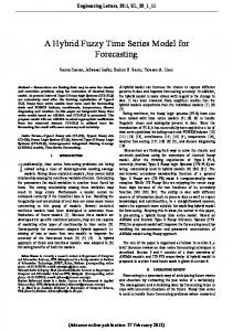
Case Structure Each stored case contains information relating to a specific situation and consists of an input profile (i.e. a vector of temperature values) together with the various fields shown in Table 1. A 40 km data profile has been found to give sufficient resolution to characterise the problem case. The parametric features of the different water masses that comprise the various oceans vary substantially, not only geographically, but also seasonally. Because of these variations it is therefore inappropriate to attempt to maintain a case base representing patterns of ocean characteristics on a global scale; such patterns, to a large extent, are dependent on the particular water mass in which the vessel may currently be located. Furthermore, there is no necessity to refer to cases representative of all the possible orientations that a vessel can take in a given water mass. Vessels normally proceed in a given predefined direction. So, only cases corresponding to the current orientation of the vessel are normally required at any one time. The strategy adopted was to maintain a centralised database in which all the thermal data tracks and satellite pictures (see Figure 4) available for all the water masses in the world, could be stored, in a condensed form, and then to retrieve from this database, transform into cases and store in the case base, the data relevant to a particular geographical location. A database composed of thousands of data profiles collected during the last decade during many oceanic voyages is maintained at PML, together with satellite images. The database is updated weekly. For the purpose of the current research a subset of the main PML database has been constructed for a region of the Atlantic Ocean situated between the UK and the Falkland Islands (in particular, between latitudes 50 to –52, and longitudes 0 to -60). Cases are constructed from the data held in the database and stored in the case base, according to the classification indicated in Table 2.

10

The case retrieval algorithms used give priority to the retrieval of the more recent cases. Spatial and temporal selection is required; a simple indexing structure has been implemented which groups cases, taking into account both their geographical and temporal proximity.

CASE RETRIEVAL From the data are recorded in real time, the input profile, I, of the problem case is created. A search is made in the case base to retrieve all cases having similar profiles. Five metrics are used to determine the similarity between the problem case and each of the retrieved cases. The metrics used in the retrieval process give priority to cases based on complementary criteria. They enable cases to be retrieved whose input profiles are similar to the problem case with respect to their temperature profiles (Metric 1 and Metric 2), general trend in temperature (Metric 3), similarity in terms of the Sobel Filter of the input profiles (Metric 4), and similarity with respect to the average sea temperature over the distance represented by the case (Average Temperature Metric).

Metric 1 The element I40 of the input profile represents the temperature at the point at which the forecast is being made. The difference between the value of I40 and each of eight equally spaced values of the input profile of the problem case are first calculated. Let these values be denoted by DIx, (x = 1, 2,… 8). Then, corresponding differences, DIAx , are calculated for the case being considered in the case base, and the difference of the differences DIx - DIAx is obtained. The eight such results are then weighted (by giving greater weight to differences relating to profile values

11

whose position is close to I40 ) and their absolute values are summed, to obtain Metric 1. The complete calculation of Metric 1 is given by

Metric _ 1 =

∑ ( (I 40 − Ii *5+1 ) − (IA 40− IA i *5+1 ) * (84 + i * 2) / 100 ) 7

i=0

where the vector Ij, (j = 1, 2 … 40) represents the input profile of the problem case and IAj, (j= 1, 2 …40) represents the input profile of the case being considered from the case base. The closer that the profiles being compared match, the smaller will be the value of Metric 1.

Metric 2 This metric is similar to the previous one, the difference being that a moving average along the input profile is calculated, using a window of four values. This metric uses the difference between I40 and each of thirteen other values of the input profile of the problem case relating to points at 3 km intervals (starting at I1 ). The values obtained are weighted and summed as in the calculation of Metric 1. This is repeated for all the cases stored in the case base. This metric gives a more general indication of the similarity between the present case and the retrieved cases than Metric 1.

Metric 3 For the problem case the difference DI between the average value of the first five input profile values and the average value of the last five input profile values is calculated. A similar difference value DIA is calculated for the stored case currently under consideration. The absolute

12

value of the difference between DI and DIA is then calculated. This process is repeated for every case in the case base. Thus:

Metric _ 3 =

5 5  5    5     ∑ Ii + 35 − ∑ Ii  / 5  −   ∑ IA i + 35 − ∑ IA i  / 5      i =1  i =1     i =1    i =1

This metric matches the general change in the water temperature in the problem case with that in each stored case being matched.

Metric 4 The Sobel filter (Gonzalez and Wintz, 1987) value is calculated for the present case and all the input profiles of the retrieved cases. The value of the Sobel Filter for a case is calculated as follows:

(∀I i: 3 < i < 38): Sobel _ I i = ((

i+2

∑ I j ) − Ii ) / 4

j =i − 2

This metric helps to identify cases from water masses having similar thermal characteristics (such as similar distribution of the temperature in the water mass and similar frequency and amplitude of oscillation of the thermal vectors).

Average Temperature Metric The Average Temperature Metric compares the average temperature, over the distance represented by each retrieved case, with that of the problem case.

13

After obtaining the value of each of the above metrics for all the cases in the Case Base, the best matching cases are determined as follows. The value of each metric is expressed on an absolute scale between 0 and 1; cases which are similar to the problem case will have a metric value close to 0; the more dissimilar the metric value of a case is from that of the problem case, the closer the value of the metric will be to 1. The best matches to the problem case are used to obtain a forecast. The best matches of each metric are then used to train a Radial Basis Function neural network (as is explained in the next section) in the adaptation stage of the reuse phase of the CBR. The metrics presented above are applied only to those cases (i) which have a date field equal to or within 2 weeks of the date field of any of the cases in obtaining the most recent forecast, or (ii) for which the geographical position differs by less than 10 km from any of the cases used to train the network in the most recent forecast.

CASE REUSE AND ADAPTATION Case adaptation is one of the most problematic aspects of the CBR cycle Most adaptation techniques are based on generalisation and refinement heuristics. In hybrid CBR systems, methods used for case adaptation include constraint satisfaction and model-based reasoning. Aamodt and Plaza (1994) outline various approaches to case-based reasoning, which differ in the way that, inter alia, they utilise the knowledge retained in past cases, and differentiate between exemplarbased reasoning, instance-based reasoning, memory-based reasoning, typical case-based reasoning and analogy-based reasoning. The approach adopted in the current research, which has some similarities with instance-based reasoning (Aha et al., 1991) is to employ a mechanism which is able to absorb the inherent knowledge stored in all the selected cases appropriate to the current problem situation and to extrapolate from them a solution. A neural network is proposed to

14

perform this function, so as to benefit from the generalising ability of neural networks. The network acts as a function that obtains representative solutions from a number of cases, these being the ones most similar to the current problem solving situation. The network does not require any human intervention and a small number of rules can be used to supervise its training.

Use of a Radial Basis Function Network The type of neural network employed is the Radial Basis Function (RBF), which has properties that make it particularly appropriate for this type of problem: such a network can be trained quickly, has very good generalising abilities (although being better at interpolating than at extrapolating), and can learn without “forgetting” by adapting its internal structure. This last property is particularly interesting in the present situation since the network is continuously being retrained, thus enabling it to learn new features within one particular water mass whilst retaining other features previously learned. Although this increases the training time, it improves the generalisation capability since at any time the forecast is based not only on the last set of retrieved cases which were used to retrain the network, but also on those cases used in the recent past which also influence the forecast. This feature contributes to the generation of a continuous, coherent and accurate forecast. The algorithm developed for the construction of the network used in the current work is a variation of the general algorithm presented by Bishop (1995). In an RBF network the input layer is a receptor for the input data. The hidden layer performs a non-linear transformation from the input space to the hidden layer space. The hidden neurons form a basis for the input vectors and the output neurons merely calculate a linear combination of the hidden neurons’ outputs. Activation is fed forward from the input layer to the hidden layer where a Basis Function, which is the Euclidean distance between the inputs and the centres of the basis function, is calculated (Fritzke, 1994). The

15

weighted sum of the hidden neuron’s activations is calculated at the single output neuron. The approach presented here automates the process of determining which centres to use and where to locate them, and guarantees a number of centres very close to the minimum number that gives optimum performance. The network is retrained before any forecast is made using the retrieved cases and the internal knowledge (weights and centres) of the network. For each metric, the k best matches are used in the adaptation phase of the CBR cycle to train the network. If the value of the metric associated with any of these two hundred cases is greater than three times the corresponding metric value of the best match, that case will not be used for training. A reasonable number k of cases is required to train the ANN. In practice a value of around 200 for k has been found to be satisfactory. If the value of k is too high, it becomes increasingly more difficult to train the network in the time available, whilst too small a value restricts the generalising ability of the neural network. Every time that the network is retrained, its internal parameter values are adapted to the new problem and the retrieved cases are adapted to produce the solution, which is a generalisation of those cases. The information from matching cases is used to create the input vector and corresponding output value used to train the network, which uses 9 input neurons, between 20 and 35 neurons in the hidden layer and 1 neuron in the output layer. The input vector values are the differences between the last temperature value (of the input profile) and each of the temperature values of the input profile at 4 km intervals. The output of the network is the difference between the temperature at the present point and the temperature 5 km ahead.

Centre and Weight Adaptation

16

Initially, twenty vectors are randomly chosen from the first training data set and used as centres in the middle layer of the RBF network. All the centres are associated with a Gaussian function, the width of which, for all the functions, is set to the mean value of the Euclidean distance between the two centres that are separated the most from each other. Training of the network is accomplished by presenting corresponding input vector values and desired output values. After an input vector activates every Gaussian unit the activations are propagated forward through the weighted connections to the output units which sum all incoming signals. The comparison of actual and desired output values enables the mean square error (the quantity to be minimised) to be calculated. The closest centre to each particular input vector is moved toward the input vector by a percentage α of the existing distance between them. Using this technique the centres are positioned close to the highest densities of the input vector data set. The aim of this adaptation is to force the centres to be as close as possible to as many vectors from the input space as possible. The value of α is initialised to a value of twenty each time that the network is retrained, and its value is linearly decreased with the number of iterations until it becomes 0; then the network is trained for a number of iterations (between 10 and 30 iterations for the whole training data set) in order to obtain the best possible weights for the final value of the centres. The delta rule (Bishop, 1995) is used to adapt the weighted connections from the centres to the output neurons. In particular, for each set of input and target output values, one delta rule adaptation step is made.

Insertion of New Units

17

A new centre is inserted into the network when the average error in the training data set does not fall more than 10% after 10 iterations (using the whole training set. Centres are deleted when they do not contribute significantly to the output of the neural network: i.e. a neuron is removed if the absolute value of its associated weight is smaller than twenty per cent of the average value of the absolute value of the five smallest weights. The number of neurons in the middle layer is maintained above 20. This is a simple and efficient way of reducing the size of the network without dramatically decreasing its memory.

Termination of Training The network is trained for a maximum of two minutes. In the real time operation a forecast is produced every 2 km (corresponding to a time of 6 minutes at a speed of 12 knots, which is the maximum speed that the vessel currently in use can attain). After travelling 2 km a new set of training cases is retrieved and the network is retrained. It has been found, empirically, that these times are sufficient to train the network and obtain a forecasting error smaller than with any other forecasting method used in the experiments. If at any point the average error obtained using the training data set becomes smaller than or equal to 0.05 °C, the training is halted to prevent the neural network from becoming over-specialised through memorising the training vectors.

CASE REVISION AND RETENTION After case adaptation a precise value is obtained for the forecasted temperature a distance of 5 km ahead of the current location. Error limits are defined and are used to revise the output of the neural network so as to produce a more realistic forecast output, in the form of an interval of

18

output values, centred on the indicated precise value. If the error limits are too wide the forecast will be meaningless; therefore a trade off is made between a broad error limit (that will guarantee that the real solution is always within its bands) and a precise solution. The expected accuracy for a prediction depends largely on two factors: the water mass in which the forecast is required, and the relevance of the cases stored in the case base for that particular prediction. For example, it can be seen in Figure 5 that between the 6000 km and 7000 km positions (equatorial waters) the temperature of the water is more stable than in the region between the 9000 km and 10000 km positions (near the Falklands Islands). Therefore a forecast produced around the equator can be assigned a smaller error interval than one obtained in the vicinity of the Falkland Islands. Each water mass is assigned a default error limit, EL0 , which has been empirically obtained. Each time that a cruise crosses a water mass, a new error limit ELz (0 < z < 6) is calculated by averaging the error in all the predictions made. If, for a certain water mass, z is equal to 5 and a vessel crosses that water mass again, the previous error limit is replaced by a new one. The error limits are used in collaboration with the average error associated with each of the cases used to train the network in obtaining a forecast. The error limit determines the interval, centred on the precise temperature value obtained from the network, and indicates that there is a probability of 90% that the forecast lies within this interval. Then, if F is the output of the network, AE is the average forecast error of the cases is used to produce a given forecast, and AEL is the average value of the error limits recorded in these cases, the error interval is defined by the expression:

[ F - ((AE*0.65)-(AEL*0.35)),

F + ((AE*0.65)-(AEL*0.35)) ]

19

The values used in this formula have been empirically obtained using data from all the water masses of the Atlantic Ocean. However, these values may not be appropriate for other oceans.

Case Retention - Learning In the last stage of the CBR cycle, the new forecasting experience is incorporated into the case base. Learning is achieved in different ways in the system. When the ship has travelled a distance of 5 km (on a straight course) after making a forecast, it is possible to determine the accuracy of that forecast, since the actual value of the parameter (e.g. sea surface temperature) for which the forecast was made can then be measured. This forecasting error is used to update the average error of all the cases that were used in producing that particular forecast. The average error field of each case used to train the neural network is continually updated, to maintain accurate error limits. Pruning the case base also contributes to the learning; cases in which the average error is very high are removed. The maximum permissible average error needs to be defined. Empirically, it has been found that for cases for which the average error attains a value of 0.12 °C, the average error never subsequently reduces to a value smaller than 0.05 °C. If the average error of a case is equal to, or higher than the 0.1 °C threshold, the case is removed from the case base. Furthermore, cases which have not been used during the previous 48 hours are deleted; so also are cases which have not been used in the previous 100 km. It is necessary to determine when the case base should be updated by creating additional cases from the database. This is done when the database receives new satellite images (once per week). If the forecasting error is greater than 0.2 °C for more than 20 predictions, additional cases are created from data stored in the data base. If, over a

20

period of operation in a particular water mass, it is found that most of the cases selected from the case base are clustered around some point a distance x, say, either ahead or behind the vessel, this suggests that the whole water mass may have moved this distance x since the data from which the cases were created were obtained. In such a situation, the operational strategy is then to utilise cases relating to this indicated area, centred on a position a distance x from the current position. The most significant aspect of learning is that due to the modification and storage of the internal structure of the neural network and its parameter values. For this purpose, the weights and centres of the network, and also the width of the Gaussian functions associated with the centres, are modified during the adaptation process and stored. Learning is a continuous process in which the neural network acts as a mechanism that generalises from the input data profiles and learns to identify new patterns. The case base may be considered to act as a long term memory since it is able maintain a huge number of cases that characterise previously encountered situations. In contrast, the stored network knowledge may be considered to behave as a short term memory for the recognition of recently learned patterns, and which enables the system to adapt to localised situations.

RESULTS The hybrid forecasting system has been tested in the Atlantic Ocean in September 1997 on a research cruise from the UK to the Falkland Islands which crossed several water masses and oceanographic fronts. Figure 1 shows the temperature values recorded by the vessel during this cruise. The average error in forecasting the temperature 5 km ahead was found to be 0.020 °C. Only 4.5% of the forecasts have an error higher than 0.5 °C, 8.33% higher than 0.04 °C and 32% higher than 0.020 °C. These figures indicate that the hybrid system is capable of producing a

21

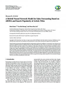
forecast with a probability of 0.96 that the error in the forecast is smaller than 0.05 °C. Although the experiments were carried out using a limited data set (over a distance of 11000 km between the latitudes 50º North and 50° South), eleven water masses with different characteristics were crossed, including six fronts. Figure 5 illustrates the error in the forecasts over a total traversed distance of 10500 km. This graph does not take into account the improvement obtained using error limits during the review phase of the CBR cycle. A similar experiment was carried out using the data recorded during the cruise (Figure 1) but this time using instances obtained from satellite images recorded more than one week before that the oceanographic data set presented in Figure 4. The experiment was carried out with 25% of the data represented in Figure 1, this limitation being due to the availability of the satellite images, and also because the computing resources available were insufficient to allow these tests to be run over the whole data set. Table 3 shows how the average errors were found to vary when satellite images of different ages were used; in particular, the table indicates that, using satellite images which are 1 or even 2 weeks old, the accuracy of the forecast is not substantially decreased. In may also be seen in Table 3 that, using pictures that are 3 or more weeks old, the forecasting error may be similar to the error obtained using pictures collected exactly one year back. This is the reason why data up to one year old is kept in the database and in the case base. If, for technical reasons (i.e. clouds covering a certain area or problems in data telecommunications), recent satellite images can not be obtained, data recorded one year back can be used by the system and may in fact produce better results than data recorded three or four weeks previously. This is due to the annual cycle of most of the water masses. However, such results can not be guaranteed, as there are also other factors that determine the pattern of ocean temperature variations.

22

Experiments were carried out to compare the performance, in terms of the average error obtained, of the hybrid system with other forecasting approaches: a Finite Impulse Response neural network (Corchado et al., 1998) a standard Radial Basis Function network (Corchado et al., 1997b), a Linear Regression model, an ARIMA (Auto-Regressive Integrated Moving Averages) model (Box and Jenkins, 1976), and a CBR system alone (Rees et al., 1996). The forecasting error using the CBR-ANN hybrid was found to be smaller than with any of the other forecasting methods. In particular, the average forecasting error outside the error limits (0.001 °C) is significantly smaller than the value obtained by any of the other forecasting methods. The standard deviation of the error is between 0.08 °C and 0.106 °C depending on the data used to create the cases. Also, the standard deviation of the error increased by more than 50% when using any of the other methods. It is important that the system does not forecast that the temperature is increasing when in fact it is decreasing and vice versa. The average percentage of such misleading forecasts is between 3% and 6% for the hybrid system, depending on the data used to create the cases. These percentages were found to increase by a factor of three when other forecasting methods were used.

CONCLUSIONS An approach to real-time forecasting has been presented that combines a case based reasoning system and an artificial neural network. The particular forecasting task addressed is difficult for two reasons: the complexity of the media in which the forecast is to be obtained and the fact that the forecast has to be made in real time. The methodology developed is capable of producing a forecast with a sufficient degree of accuracy and within the time constraints imposed by the real time nature of the problem. Although the accuracy of the forecast depends to a large extent

23

on the quality of the cases and when those cases have been collected, it has been shown that a good quality forecast can be obtained even with data collected one year before the forecast is made. The RBF neural network plays an important role in the system; it adapts its structure in an unsupervised way to the characteristics of the environment and draws on the information held in matching cases of previous forecasting experience to generate a new forecast, representative of them all. The results obtained may be extrapolated to obtain a forecast a further distance ahead of the current location. The further ahead that the point is for which the forecast is made, the more unreliable will be the forecast, as is shown in Table 4. The limitations of this method of forecasting are as follows. (i) The present system is not able to create a forecast while the vessel is changing its trajectory (or has changed it in the last 40 km). However, the structure of the system could be modified to enable it to forecast in such situations. (ii) The system, in its present form, can operate effectively only if there are no large discontinuities in the data. If this is not the case it has been found that forecasts can still be obtained, but only if the discontinuity is no greater than around 5 km. (iii) The system can not be expected to work in an area for which there are no previous cases; in such a situation the only way forward is to use a back-up system, for which it is believed that a Finite Impulse Response network model (Corchado et al., 1998) may be the most appropriate. In conclusion, the proposed forecasting method employs the ability of case-based reasoning to index, organise and retrieve relevant data, together with the generalisation, learning and adaptation capabilities of a radial basis function neural network, and thus, by integrating the neural network within the CBR cycle of operations, combines the strengths of both connectionist and symbolic

24

techniques. It is believed that this approach may potentially be applicable to other forecasting situations in other domains.

ACKNOWLEDGEMENTS The contributions of N. Rees and Prof. J. Aiken at the Plymouth Marine Laboratory in the collaborative research presented in this paper are gratefully acknowledged.

REFERENCES Aamondt, A. and Plaza, E. 1994. Case-Based Reasoning: foundational issues, methodological variations, and system approaches. AI Communications, 7 (1): March. Aha, D., Kibler, D. and Albert, M.K. 1991. Instance-based learning algorithms. Machine Learning 6(1). Bishop, C. R. 1995. Neural Networks for Pattern Recognition. Oxford: Clarendon Press. Box, G.E.P. and Jenkins, G.M. 1976. Time Series Analysis: Forecasting and Control. Revised ed. San Francisco: Holden-Day. Corchado, J., Rees, N., Lees, B. and Fyfe, C. 1997a. Study and comparison of multi-layer perceptron NN and radial basis function NN in oceanographic frontal warning. In Procs. Application and Science of Artificial Neural Networks, SPIE International Symposium an Aerospace/Defense Sensing and Control, April, Orlando, Florida Corchado, J., Lees, B., Fyfe, C. and Rees, N. 1997b. Adaptive agents: learning from the past and forecasting the future. In Procs. 1st International Conference on Knowledge Discovery and Data Mining, April, London. Cochado, J., Fyfe, C. and Lees, B. 1998. Unsupervised neural network for temperature forecasting. In Procs. EIS’98, February, Tenerife, Spain. Fritzke, B. 1994. Fast Learning with Incremental RBF Networks. Neural Processing Letters. 1:2-5. th Goel, A. 1991. A model-based approach to case adaptation. In Procs. 13 Annual Conf. of the Cognitive Science Society. Erlbaum. Gonzalez, R. and Wintz, P. 1987. Digital Image Processing, 2nd ed. Addison Wesley. Hunt, J. and Miles, R. 1994. Hybrid case-based reasoning. The Knowledge Engineering Review. 9(4): 383-397. Kolodner, J. 1993. Case-Based Reasoning. San Mateo, CA: Morgan Kaufmann. Lees, B., Rees, N. and Aiken, J. 1992. Knowledge-based oceanographic data analysis. In Procs. Expersys-92. ed. F. Attia, A. Flory, S. Hashemi, G. Gouarderes, J. Marciano. 561-65, October, Paris: IITT International. Lees, B. and Corchado, J. 1997. Case-based Reasoning in a hybrid agent-oriented system.In Procs. Fifth German Workshop on Case-Based Reasoning - Foundations, Systems and Applications. March, Bonn. López de Mántaras, R. and Plaza, E. 1997. Case-Based Reasoning: an overview. AI Communications 10:21-29, IOS Press. Nakhaeizadeh, G. 1994. Learning prediction of time series: a theoretical and empirical comp arison of CBR with some other approaches. In Topics in Case-Based Reasoning. First European Workshop on Case-Based Reasoning (EWCBR'93), ed. S. Wess, K.-D. Althoff, and M.M. Richter, Berlin: Springer Verlag.

25

Pankratz A. 1991 Forecasting with Dynamic Regression Models, Wiley Series in Probability and Mathematical Statistics. Addison-Wiley. Rees, N., Aiken, J. and Corchado, J. M. 1996. Internal Report on CBRs and Oceanographic Forecasting, September, Plymouth, U.K.: PML. Riesbeck, C. K. and Schank, D. B. 1989. Inside Case Based Reasoning. Erlbaum. Roderman, S. and Tsatsoulis, C. 1993. PANDA: a case-based system to aid novice designers. AI EDAM, 7(2):125-134. Teague, W. J., Carron, M. J. and Hogan P. J. 1990. A Comparison between the generalised digital environmental model and levitus climatologies. Journal of Geophysical Research. 95(C5):7167-7183, May. Tomczak, M. and Godfrey, J. S. 1994. Regional Oceanography: An Introduction. New York: Pergamon. Watson, I., and Marir, F. (1994). Case-based reasoning: a review. The Knowledge Engineering Review, 9(4):355381. Weigend, A. S. and Gershenfeld, N. A. 1995. Time Series Prediction: Forecasting the Future and Understanding the Past, Santa Fe Institute Studies in the Sciences of Complexity, Addison-Wiley. Wilke, W. and Bergmann, R. 1996. Incremental adaptation with the INRECA system. In Procs. ECAI 1996. Workshop on Adaptation in Case-Based Reasoning.

26

Table 1. Case structure Case Field

Explanation

Identification

unique identification: a positive integer in the range 0 to 64000

Input Profile, I

a 40 km temperature input vector of values Ij, (where j = 1, 2, … 40) representing the structure of the water between the present position of the vessel and its position 40 km back

Output Value, F

a temperature value representing the water temperature 5 km ahead of the present location

Source

data source from which the case was obtained (satellite image or data track); each source is identified by its acquisition date, time and geographical coordinates

Time

time when recorded (although redundant, this information helps to ensure fast retrieval)

Date

date when the data were recorded (included for the same reasons as for the previous field)

Location

geographical co-ordinates of the location where the value I40 (of the input profile) was recorded

Retrievals Tally

number of times the case has been retrieved to train the neural network (a non-negative integer)

Orientation

approximate direction of the data track, represented by an integer x, (1 ≤ x ≤12)

Retrieval Time

time when the case was last retrieved

Retrieval Date

date when the case was last retrieved

Retrieval Location

geographical co-ordinates of the location at which the case was last retrieved

Average Error

average error over all forecasts for which the case has been used to train the neural network

27

Table 2. Case classification and construction Classification

Description

1

Cases within an area delimited by a circle of radius P km centred on the present position of the vessel. i.e. P = X+(X*0.25). Where: •

X is the distance between the present position of the vessel and the geographical position of the case with a retrieval field equal to 4 and in which the averaged error is smaller than 0.05 and which has been retrieved within the last 20 km or 24 hours. If there is no case with a retrieval field equal to 4, the one having a value closest to 4 will be chosen. These threshold values have been obtained in experiments carried out with data sets obtained in AMT cruises.

•

25 ≤ P ≤ 200

2

Cases with the same orientation as the present cruise track.

3

Cases from data recorded during the same month as the cases that are stored in the case base in which the forecasting error is less than 0.05 and which have been used during the last 24 hours or 50 km. Cases are also constructed from data recorded in the previous month under the same conditions.

4

Cases constructed from data recorded during the last two weeks.

28

Table 3. Average error in the forecast outside the error limits for satellite images of different ages Time interval between the image being recorded and the real time data being recorded (number of weeks)

Average Error (°C)

1

0.020

2

0.024

3

0.034

4

0.048

52

0.033

29

Table 4. Average forecasting error at different distances Forecast Distance (km)

Average error (hybrid system) (°C)

Average error (hybrid system) using confidence limits (°C)

5

0.02

0.001

10

0.05

0.01

15

0.13

0.06

20

0.26

0.11

30

Captions for Figures

Figure 1. Thermal data profile, recorded in September 1997 by a research vessel travelling from the U.K. to the Falkland Islands.

Figure 2. Hybrid CBR-ANN system outline.

Figure 3. Hybrid system control flow.

Figure 4. (a) Satellite image, (b) a track obtained from satellite image.

Figure 5. Absolute value of the forecasting error (°C) using the hybrid system.

31

32

Problem Case (created in real time)

Data Acquisition

Retrieved Cases

Cases Cases generated from satellite images and real time data

Retrieve

Case Base

New Forecast Case, New case Revised Network ANN weights Parameters & centres

ANN weights & centres

Reuse

Data Store

Retain Error limits

Revised Forecast

Revise

33

Proposed Forecast

Database of Real Time Ocean Data (Recorded at one minute intervals)

Database of Satellite Images (updated weekly)

Retrieve

Retrieve Retrieve Calculate forecast error

Case Problem case

Case Base

Error

Create Problem

Create historical cases

Compare with stored cases

k revised cases

Retrieve

Save Retrieve most relevant cases Database of previous forecasts Training

k matching cases Save

Retrieve parameters ANN

Error limits

Knowledge Base: Weights Centres

Stop Proposed Training Forecast

Retrieve

Save Update parameters Case Base

Retain

Final Forecast

Reuse

Revise

34

35

(a)

Temp (oC)

Distance (km)

(b)

36

0.7 0.6 Error 0.5 (oC) 0.4 0.3 0.2 0.1 0 500

1500

2500

3500

4500 5500 6500 Distance (km)

37

7500

8500

9500 10500