A hybrid feature selection method based on binary state transition

This article has been accepted for publication in a future issue of this journal, but has not been fully edited. Content may change prior to final publication. Citation information: DOI 10.1109/JBHI.2018.2872811, IEEE Journal of Biomedical and Health Informatics 1

A hybrid feature selection method based on binary state transition algorithm and ReliefF Zhaoke Huang, Chunhua Yang, Member, IEEE, Xiaojun Zhou, and Tingwen Huang, Member, IEEE

Abstract—Feature selection problems often appear in the application of data mining, which have been difficult to handle due to the NP-hard property of these problems. In this study, a simple but efficient hybrid feature selection method is proposed based on binary state transition algorithm (BSTA) and ReliefF, called ReliefF-BSTA. This method contains two phases: the filter phase and the wrapper phase. There are three aspects of advantages in this method. First, an initialization approach based on feature ranking is designed to make sure that the initial solution is not easy to get tapped into local optimum. Then a probability substitute operator based on feature weights is developed to update the current solution according to the different mutation probabilities of the features. Finally, a new selection strategy based on relative dominance is presented to find the current best solution. The simple and efficient algorithm k-Nearest Neighborhood (k-NN) with the leave-one-out cross validation is used as a classifier to evaluate feature subset candidates. The experimental results indicate that the proposed method is more efficient in terms of the classification accuracy through a comparison to other feature selection methods using seven public datasets and several real biomedical datasets. For public datasets, the proposed method improved the classification average accuracy by about 2.5% compared with the filter method. For a specific biomedical dataset AID1284, the classification accuracy significantly increased from 77.24% to 85.25% by using the proposed method. Index Terms—Feature selection, Hybrid method, State transition algorithm, ReliefF

I. I NTRODUCTION N the past decade, the data in the world have had an drastically increase and we have lived in an era of big data. In this environment, with the challenge of “rich data without knowledge”, how to find useful information from datasets has become a problem needed to address urgently. The emergence of data mining provides strong technical support for the urgent need. It is the process of obtaining the hidden useful information from a great number of data through a variety of algorithms [1]. However, in many applications, a dataset may contain redundant, irrelevant and relevant features that bring in high computational complexity and poor learning performance [2]. Especially in biomedical and health informatics, the situation becomes much worse because there exist a lot of features in the datasets [3], [4], [5], [6], [7], [8]. For instance, in computer-aided detection (CADe) of polyps in computed tomography (CT) colonography, a common approach to classification in a CADe scheme is to

I

Z. Huang, C. Yang and X. Zhou are with the School of Information Science and Engineering, Central South University, Changsha 410083, China e-mail: [email protected]. T. Huang is with Texas A&M University at Qatar, Doha 23874, Qatar.

extract many texture, gray-level-based, geometric, and other features based on domain knowledge. However, not all of these extracted features might be helpful in discriminating lesions from nonlesions. Therefore, in the design of an effective classifier, it is critical to select the most discriminant features to differentiate lesions from nonlesions. Under this circumstance, feature selection is an effective technique to handle these problems [9]. Its goal is to find the most proper feature subset from the original feature set which makes the constructed model better. Feature selection brings two benefits to data modeling. For one thing, feature selection can eliminate the irrelevant or redundant features so as to simplify the learned model and reduce the training time. For another, it can find the truly useful features that improve the accuracy of the model and make it easy for researchers to understand the process of data generation. However, finding the truly relevant features is challenging due to two reasons: (i) the huge search space, that is, an n-dimensional dataset has 2n feature subsets and it is not possible to search the entire solution space for a large n; (ii) the complex interactions among features, which makes hard to distinguish which features are useful and which ones are useless. Hence, feature selection is an NP-hard combinatorial problem. At present, there exist many methods to handle the feature selection problem, which can be grouped into two main categories, i.e., the filter method and the wrapper method [2]. For the first category, filter based feature selection method relies on data-dependent criteria to evaluate features individually or in feature subsets without involving any data mining algorithm. Representative filter based feature selection method includes correlation coefficient [10], Gini index [11], F-score criterion [12], minimum-redundancy maximum-relevancy (mRMR) [13], ReliefF [14], correlation-based feature selection (CFS) [15] and so on. The advantage of the filter method is that it consumes less computational resources, while it has the downside of less effective without considering the influence of a classifier. For the second category, wrapper based feature selection method treats the selection of the feature subset as an optimization problem. They first generate some different feature subsets and evaluate these subsets. Then the current best feature subset are selected among them through comparison. The final best feature subset is found until the termination criterion is met. Representative wrapper based feature selection method includes sequential forward selection (SFS) [16], sequential backward selection (SBS) [17], sequential forward floating selection (SFFS) and sequential backward floating selection (SFBS) [18]. Unfortunately, the

2168-2194 (c) 2018 IEEE. Personal use is permitted, but republication/redistribution requires IEEE permission. See http://www.ieee.org/publications_standards/publications/rights/index.html for more information.


main drawback of these methods is that it is more often to obtain the local optimal solution. To address the drawbacks of traditional wrapper approaches, researchers have also applied evolutionary computation (EC) techniques, including genetic algorithms (GAs)[19] , genetic programming (GP) [20] , particle swarm optimization (PSO) [21] and ant colony optimization (ACO) [22] to feature selection problems. The advantage of the wrapper method is that it is more effective on the classification accuracy, but it consumes a large amount of time [23]. To summarize, both the filter method and the wrapper method have advantages as well as disadvantages. It is promising to combine these two methods into a hybrid one by making use of each other’s strengths. Recently, a novel nature-inspired method called state transition algorithm (STA) has emerged in global optimization by the co-authors of this paper [24]. The powerful global search ability and flexibility of state transition algorithm have been demonstrated in many real-world applications [25], [26], [27], [28], [29], [30], [31], [32], [33], [34], [35]. In addition, ReliefF is a widely used filter based feature selection method in handling the feature selection problem [14]. In this study, a hybrid feature selection method named ReliefF-BSTA is proposed based on binary state transition algorithm (BSTA) and ReliefF to solve the feature selection problem. First, the ReliefF is applied to provide some useful features that are helpful to classification. However, the limitation of the ReliefF is that it cannot effectively remove redundant features. Hence, in the next wrapper stage, these features are used as candidates, which are further optimized by the BSTA. The simple and efficient algorithm k-Nearest Neighborhood (kNN) is used to evaluate the robustness, efficiency, and accuracy of the hybrid feature selection technique. The novelty and main contributions of the proposed method are highlighted as follows: •

•

•

•

An initialization approach based on feature ranking is proposed in the wrapper stage, which not only reserves some top-ranked features, but also makes the initial solution not easily get trapped into local optimum. A probability substitute operator based on feature weights is developed to update the current solution. Since the mutation rate function is a bell-shaped curve, mutation probability of each feature is different. So, the proposed algorithm has better global convergence and stronger robustness performance. For the sake of reducing the computational complexity, a new selection strategy named relative dominance-based selection is proposed to evaluate the candidate solutions. A comparison experiment is conducted between the ReliefF-BSTA and other metaheuristic-based methods.

The rest of paper is organized as follows. Section II gives a brief review of feature selection, ReliefF, and BSTA. Section III presents the proposed hybrid feature selection method. Section IV describes the efficiency of the proposed method via experimental results. Finally, Section V concludes the paper.

x

1

0

1

1

0

1

0

0 Y=Selected

Features N=Not Selected Y Y

Y

Y N

N

N N

Fig. 1: A binary encoding 8-dimensional vector x

II. P RELIMINARIES A. Problem statement of feature selection Given a dataset consisting of m samples and n features, D is a set that contains all features. Feature selection aims to find d features from D so that the process of model construction is fast and best. That is, the aim of feature selection is to find a best feature subset from D, which can maximize the classification accuracy with the minimal number of features. In this study, the binary encoding vector x is used to denote a solution of the feature selection problem, which is described as follows: x = (x1 , x2 , ..., xn ), xi ∈ {0, 1}, i = 1, 2, ..., n

(1)

where xi = 1 means that the ith feature is selected, whereas xi = 0 means that the feature is not selected. Fig. 1 illustrates an 8-dimensional vector x. Here the solution x = [1, 0, 1, 1, 0, 1, 0, 0] represents the corresponding selected 1st, 3rd, 4th and 6th features. According to the above description, the feature selection problem can be expressed as the following form: max f1 = Acc(x) min f2 = ||x||0 s.t.

x = (x1 , x2 , ..., xn ), xi ∈ {0, 1}, i = 1, 2, ..., n 1 ≤ ||x||0 ≤ n

(2)

where Acc(x) represents the classification accuracy of the model constructed according to the corresponding x. ||x||0 stands for the number of the selected features in x. Obviously, Eq. (2) is a constrained multiobjective optimization problem. However, the feature selection problem has its own characteristics. Because our intention is to improve the classification accuracy of the model. Hence, the first objective is the primary goal. So, this problem is not a general constrained multiobjective problem. B. A brief introduction to ReliefF ReliefF is a widely used filter based feature selection method that finds the best feature subset by calculating the features’ weights. The Relief algorithm was firstly proposed by Kira in 1992 [36], which is initially confined to two-class classification problems. This algorithm is a feature weighting algorithm, which assigns different weights to features according to the correlations between features and categories. The feature whose weight is greater than an artificial threshold will be selected. The correlation between features and categories in the Relief algorithm is based on the distinguishing ability of



features to the close-range samples. Since the Relief algorithm is relatively simple, efficient and can produce the satisfactory results, it has been widely used. However, a key limitation of the Relief algorithm is that it can only handle two-class classification problems. To address this problem, ReliefF was proposed by Kononenko in 1994 [14], which can handle multiclass problems. When handling multiclass problems, given that the class labels of the training dataset is C = {c1 , c2 , ..., cl } , a sample Ri is first randomly selected from the training dataset by the ReliefF. Then it searches for k nearest neighbors (called near Hits) of Ri from the same class, which is denoted by Hj (j = 1, 2, ..., k), and also k nearest neighbors (called near Misses) of Ri from different classes, which is denoted by Mj (c)(j = 1, 2, ..., k). Finally, this algorithm repeats these two steps m times. The weight of feature A is updated as:

W (A) = W (A) −

k ∑

diff(A, Ri , Hj )/(m ∗ k)+

j=1

∑

∑ p(c) diff(A, Ri , Mj (c))]/(m ∗ k) 1 − p(class(R)) j=1 k

[

c̸∈class(R)

(3) where m is the number of iterations. diff(A, R1 , R2 ) means the difference between the sample R1 and the sample R2 in the feature A, and it is defined as:       diff(A, R1 , R2 ) =

    

|R1 [A]−R2 [A]| max(A)−min(A) ,

0, 1,

if A is continuous if A is discrete and R1 [A] = R2 [A] if A is discrete and R1 [A] ̸= R2 [A] (4)

1

1

0

1

0

swap(2,3)

1

1

0

1

1

0

1

Fig. 2: Illustration of swap transformation

1

1

0

1

0

shift(3,5)

1

1

1

1

0

0

1

Fig. 3: Illustration of shift transformation where xk ∈ Zn represents a current state, that is, a solution. uk represents historical states. Ak (.) and Bk (.) are transfor⊕ mation operators, which stand for state transition matrixes. is defined as an operator performed on two states. f is the fitness function. There are four special state transformation operators developed for generating candidates for both local and global search. 1) Swap transformation: xk+1 = Aswap (ma )xk , k

(6)

where, Aswap ∈ Rn×n is a swap transformation matrix, k and ma is a swap transformation factor that is a constant integer. Fig. 2 gives the illustration of swap transformation. Under this circumstance, the expression is given as follows:        

1 0 1 1 0 1





      =      

1 0 0 0 0 0

0 0 1 0 0 0

0 1 0 0 0 0

0 0 0 1 0 0

0 0 0 0 1 0

0 0 0 0 0 1





      ×      

1 1 0 1 0 1

       

2) Shift transformation: C. A brief introduction to binary state transition algorithm Binary state transition algorithm (BSTA), the binary variant of discrete state transition algorithm (DSTA), is a new intelligent optimization algorithm for solving boolean integer optimization problems [26]. The DSTA is the discrete variant of state transition algorithm (STA) for integer optimization problems. The STA was firstly proposed by Zhou in [24] for continuous optimization problems, which was inspired by state space representation from control theory. The main idea of STA is to generate some candidate solutions through several intelligent search operators and to reserve the current best solution by evaluating the candidates. A candidate solution is described as a state, and the transformation to update the solution is treated as a state transition. Unlike GA or PSO, STA is an individual-based optimization approach and generates candidates by using state transformation with both local and global operators alternatively. In general, the unified form of solution generation in the DSTA can be expressed as follows: { ⊕ xk+1 = Ak (xk ) Bk (uk ) (5) yk+1 = f (xk+1 )

t xk+1 = Ashif (mb )xk , k

(7)

t where, Ashif ∈ Rn×n is a shift transformation matrix, k and mb is a shift transformation factor that is a constant integer. Fig. 3 gives the illustration of shift transformation. Under this circumstance, the expression is given as follows:

       

1 1 1 0 0 1





      =      

1 0 0 0 0 0

0 1 0 0 0 0

0 0 0 0 1 0

0 0 1 0 0 0

0 0 0 1 0 0

0 0 0 0 0 1





      ×      

1 1 0 1 0 1

       

3) Symmetry transformation: xk+1 = Asym (mc )xk , k

(8)

where, Asym ∈ Rn×n is a symmetry transformation k matrix, and mc is a symmetry transformation factor



1

1

0

1

0

symmetry(2,5)

1

1

0

1

0

1

Algorithm 1 Discrete state transition algorithm 1: repeat 2: Best ← swap(Best, ∗) 3: Best ← shif t(Best, ∗) 4: Best ← symmetry(Best, ∗) 5: Best ← substitute(Best, ∗) 6: until the specified termination criterion is met 7: Best∗ ← Best

1

Fig. 4: Illustration of symmetry transformation

1

1

0

1

0

substitute(2)

1

1

0

0

1

0

1

Fig. 5: Illustration of substitute transformation

that is a constant integer. Fig. 4 gives the illustration of symmetry transformation. Under this circumstance, the expression is given as follows:        

1 0 1 0 1 1





      =      

1 0 0 0 0 0

0 0 0 0 1 0

0 0 0 1 0 0

0 0 1 0 0 0

0 1 0 0 0 0

0 0 0 0 0 1





      ×      

1 1 0 1 0 1

       

4) Substitute transformation: xk+1 = Asub k (md )xk ,

(9)

where, ∈ R is a substitute transformation matrix, and md is a substitute transformation factor that is a constant integer. Fig. 5 gives the illustration of substitute transformation. Under this circumstance, the expression is given as follows: Asub k

       

1 0 0 1 0 1



n×n



      =      

1 0 0 0 0 0

0 0 0 0 0 0

0 0 1 0 0 0

0 0 0 1 0 0

0 0 0 0 1 0

0 0 0 0 0 1

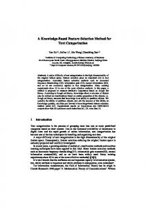
to evaluate feature subset candidates. The hybrid method not only ensures high classification accuracy, but also overcomes the limitations of slow computation. A flowchart of the proposed hybrid feature selection method is shown in Fig. 6 and the pseudocodes can be described in Algorithm 2. It works in two phases: 1) The filter phase: In this phase, the feature ranking and feature weights are calculated by using ReliefF, which are provided to the next wrapper phase. 2) The wrapper phase: A wrapper approach BSTA is designed in which BSTA selects a best feature subset containing most relevant and non redundant features based on important information about features (feature ranking and feature weights) found in the previous phase, by assessing the classification accuracy of each feature subset using k-nearest neighbor (k-NN) learner.





      ×      

1 1 0 1 0 1

       

The main procedure of discrete state transition algorithm is described in Algorithm 1. Where swap(.), shif t(.), symmetry(.) and substitute(.) are transformation operator functions. Best represents a candidate solution. Best∗ represents a current best solution. III. T HE PROPOSED HYBRID FEATURE SELECTION METHOD : R ELIEF F-BSTA A. Overview of the proposed method In this study, for higher classification accuracy and lower computational resources, a hybrid feature selection method is presented, where a filter approach ReliefF effectively reduces the large search space and provides important information about features (feature ranking and feature weights) to the BSTA, and the wrapper approach BSTA searches for the best feature subset based on feature ranking and feature weights. The k-nearest neighbor (k-NN) approach is used as a classifier

B. Feature ranking and feature weights using ReliefF The original feature set from the training dataset contains both sensitive and redundant features. If the wrapper method is directly used to find the best feature subset from the original feature set, the search space will be so large that computational cost would be high. Therefore, for the sake of reducing the search space and improving computing efficiency, ReliefF is used to evaluate the weight of each feature and sort features in terms of the feature weights. The ranking of features are denoted by f : x → S(x) and the feature weights are denoted by W = {w1 , w2 , ..., wn }. For example, if the feature x1 ranks no. 7, S(x1 ) = 7. This important information is used as references for the next wrapper method. Thus, the number of features can be decreased in the next wrapper phase, which are selected from the original feature set. After the ReliefF processes, feature weights will be normalized to [0, 1] since it is very useful to the next wrapper method. The normalization expression is given as follows: wi′ =

wi − min(wi ) max(wi ) − min(wi )

(10)

where wi′ is the normalized value. wi is the value of the original feature weight i. min(wi ) and max(wi ) are minimum value and maximum value of feature weight wi , respectively. C. Initialization based on feature ranking The way of initialization of the BSTA has an important role in this approach. Since a key limitation of the ReliefF algorithm is that it cannot effectively remove redundant features, an initialization approach based on feature ranking is



Feature weights

Dataset (N×M)

x Filter

low

0

high

1

0

0 0

1

0

0

1

1 1

1

The mutation rate of each xi

Calculate features ranking and feature weights by using ReliefF

Normalize feature weights

Fig. 8: The illustration of a function about r and w′ when t=1 and T=100

Wrapper Initialization based on features ranking Probability substitution based on feature weights Feature subset candidate

Learn the model by using kNN

No

Get the best feature subset through relative dominancebased selection

Stopping condition

D. Probability substitute operator based on feature weights Yes

The optimal feature subset

Fig. 6: A flowchart of the proposed hybrid feature selection method Length=n*pct

1

x

0

...

1

0

1

...

0

The probability of selecting a feature is q in this interval

Fig. 7: The proposed initialization approach proposed in this subsection. On the one hand, we expect that the features whose weights are higher are not all selected, since there are some redundant features among them. On the other hand, we do not expect the initial solution easily trapped into local optimization. Hence, the initialization approach is described as follows: xi = { xi =

1, 0,

In order to improve the diversity of BSTA without compromising with the solution quality, a probability substitute operator based on feature weights is proposed in this subsection, which could explore unknown areas of the search space on the basis of feature ranking by { 1 − xi , if rand() ≤ ri xi = (13) xi , otherwise

Length=n*(1-pct)

The probability of selecting a feature is p in this interval

{

q) to control the generation of the initial solution. pct ∈ [0, 1] represents the percentage of the features whose weights are greater than a certain threshold, n represents the number of features and n∗pct is the number of features that are sensitive. p ∈ (0, 1) indicates the probability of choosing a feature at which the feature has higher weight. So, a value of p is close to 1. On the contrary, q ∈ (0, 1) stands for the possibility of selecting a feature whose weight is lower.

if rand() < p , when S(xi ) ≤ n ∗ pct (11) otherwise

1, if rand() < q , when S(xi ) > n ∗ pct (12) 0, otherwise

Fig. 7 shows an outline of the proposed initialization approach. There are three user-specified parameters (pct, p, and

ri = (0.2 +

−0.2 × (t − 1) 1 )× T 1 + |wi′ − 0.5|1.6

(14)

where ri is the mutation rate of xi , which is influenced by three factors: the weight of xi , iteration t and the total number of iterations T . The value of ri decreases with the increasing of iteration t. Fig. 8 shows the illustration of a function about r and w′ . E. Relative dominance-based selection As described in Section II-A, the feature selection problem is not a general constraint multiobjective problem, which has two main conflicting objectives. However, the first objective is our primal intention whether the second objective is best or not. To reduce the computational complexity, a relative dominance-based selection strategy is presented to seek the current optimal feature subset in this subsection, based on the following definitions: Definition 1 (Feasible region): The solution space that satisfies all the constraints is called the feasible region. Definition 2 (Relative dominate): For two objectives f1 and f2 , the solutions x1 and x2 are in the feasible region, and



Algorithm 2 Pseudocode of ReliefF-BSTA 1: 2: 3: 4: 5: 6: 7: 8: 9: 10: 11: 12: 13: 14: 15: 16: 17:

The filter phase: Calculate features ranking and feature weights using ReliefF; Normalize feature weights using Eq. (10); The wrapper phase: Get the initial solution using Eqs. (11) and (12); Get the best solution so far; repeat Get the candidate solutions using Eq. (6); Update the best solution so far using Defn. (2); Get the candidate solutions using Eq. (7); Update the best solution so far using Defn. (2); Get the candidate solutions using Eq. (8); Update the best solution so far using Defn. (2); Get the candidate solutions using Eqs. (13) and (14); Update the best solution so far using Defn. (2); until the specified termination criterion is met Return the best solution

TABLE I: Datasets used in benchmark test Dataset

# of features

# of samples

# of classes

Ionosphere

34

351

2

Segmentation

19

2310

7 2

Sonar

60

208

Vehicle

18

94

4

Vowel

10

990

11

WDBC

30

569

2

Wine

13

178

3

TABLE II: Parameter settings Comparative algorithm

Parameter P opulation = 20

SGA

The mutation probability, p1 = 0.1 The crossover probability, p2 = 0.6 P opulation = 20

BPSO

The acceleration coefficients, c1 = c2 = 2 The inertia weight, w = 1

if the solution x1 is better than the solution x2 when any of the following condition holds: (1) f1 (x1 ) < f1 (x2 ); (2) f1 (x1 ) = f1 (x2 ) and f2 (x1 ) < f2 (x2 ), we call that x1 ‘relatively dominate’ x2 . Definition 3 (Relative-optimal solution): In the feasible region, the solution x is called relative-optimal solution if none of other solutions ‘relatively dominate’ it. For feature subset candidates, each of them is first used to compare with the current best feature subset according to Defn. (2). Then, if one of them relatively dominates the current best feature subset, this candidate overwrites it, else the current best feature subset is unchanged. Hence, according to Defn. (3), the only one optimal solution x can be found from the feasible region in this problem.

IV. E XPERIMENTS In this section, we will first use several well-known datasets to illustrate the performance of the proposed method ReliefFBSTA. Then the ReliefF-BSTA will be applied to a real biomedical case. In this study, seven kinds of algorithms are selected to compare with the ReliefF-BSTA, which are sparsity based method (Lasso) [37], minimum redundancy maximum relevance (mRMR) [38], ReliefF [14], the method based on genetic algorithm (SGA) [19], the method based on particle swarm optimization (BPSO) [39], and the method based on firefly algorithm (BFFA) [40]. The simple and efficient algorithm k-Nearest Neighborhood (k-NN) with the leaveone-out cross validation is used as a classifier to evaluate feature subset candidates. We set k = 1 for all the comparative algorithms in the experiments, which was also adopted in a variety of literatures [39], [19]. In the experiments, a datum from a dataset is first selected as the testing sample, and the rest constitute the training samples. All experiments are implemented on a personal computer with Intel Core i7 Duo CPU 2.8 GHz and 16 GB RAM using MATLAB.

BFFA

P opulation = 20 γ = 1.0, α = 0.5, βmin = 0.2

ReliefF-BSTA

SE = 20 pct = 0.5, p = 0.9, q = 0.1

A. Benchmark test 1) Datasets and Parameter settings: Seven datasets are selected from UCI [41] for our experiment and Table I displays concise information of these datasets. The number of features in these datasets is in the range of increasing from 13 to 60. In order for all algorithms to perform fairly for the experimental datasets, the values of the related parameters are set according to their corresponding literatures. Table II shows the detailed parameter settings of the four algorithms, except for the termination condition. To be fair, the termination condition is set as the maximum number of evaluations, which is 1000 for all datasets. Since the BSTA belongs to the individualbased algorithm and the other three algorithms belong to the population-based algorithm, SE is used to represent the number of generated candidate solutions, that is why it is called search enforcement in this experiment. 2) Experimental results: In this subsection, the ReliefFBSTA is used to compare with Lasso, mRMR, ReliefF, SGA, BPSO and BFFA on handling the feature selection problems from seven public datasets. Each algorithm runs 30 times on each dataset, and the average results are obtained from all these runs. In order to demonstrate the performances of each algorithm, two indicators, the classification accuracy (Acc) and the number of the selected features (d), are used in this paper. Table III shows the best solutions obtained by these algorithms in terms of the two indicators, Acc∗ and d∗ . Table III reports that: 1) for the Vowel, Wine, Vehicle and Segmetation, the performance of BFFA is same as that of the ReliefF-BSTA; 2) for all seven datasets, the ReliefF-BSTA achieves the best



TABLE III: The best solutions obtained by the seven algorithms Dataset

Lasso

mRMR

ReliefF

TABLE IV: Average results obtained by the seven algorithms Lasso

Dataset

mRMR

ReliefF

d

Acc(%)

d

Acc(%)

d

Acc(%)

13

99.29

9

99.29

11

99.29

d∗

Acc∗ (%)

d∗

Acc∗ (%)

d∗

Acc∗ (%)

Vowel

13

99.29

9

99.29

11

99.29

Wine

8

96.07

12

96.63

11

98.31

Wine

8

96.07

12

96.63

11

98.31

Vehicle

7

72.34

14

64.89

7

72.34

24

96.13

Vowel

Vehicle

7

72.34

14

64.89

7

72.34

WDBC

29

95.78

5

95.78

WDBC

29

95.78

5

95.78

24

96.13

Ionosphere

33

90.88

10

93.45

9

93.73

Ionosphere

33

90.88

10

93.45

9

93.73

Segmentation

17

97.79

14

97.79

11

97.88

Segmentation

17

97.79

14

97.79

11

97.88

Sonar

48

86.06

20

89.42

36

Sonar

48

86.06

20

89.42

36

88.46

Dataset

SGA

BPSO

BFFA

SGA

Dataset

BPSO

d

Acc(%)

d

Vowel

9

99.70

Wine

5

95.51

88.46 BFFA

Acc(%)

d

Acc(%)

9.00

99.70

9.00

99.70

8.24

98.87

8.00

99.55

d∗

Acc∗ (%)

d∗

Acc∗ (%)

d∗

Acc∗ (%)

Vowel

9

99.70

9

99.70

9

99.70

Wine

5

95.51

8

100

8

100

Vehicle

7

72.97

8.80

73.64

7.30

75.96

Vehicle

7

73.52

8

74.70

7

77.66

WDBC

12

93.95

13.35

97.15

13.9

98.06

7

94.70

13.80

94.81

12.7

96.09

WDBC

12

94.38

13

98.07

14

98.29

Ionosphere

Ionosphere

7

95.44

13

96.58

12

96.87

Segmentation

8

92.95

11.54

97.98

11.0

98.11

Segmentation

8

92.95

12

98.27

12

98.27

Sonar

24

95.49

29.70

92.73

29.80

95.08

Sonar

24

95.67

29

95.12

29

96.63

ReliefF-BSTA

ReliefF-BSTA

Dataset

d

Acc(%)

Vowel

9.00

99.70

99.70

Wine

8.20

99.66

8

100

Vehicle

7.20

76.01

Vehicle

7

77.66

WDBC

12.10

98.24

WDBC

11

98.42

Ionosphere

13.53

96.18

Ionosphere

11

96.87

Segmentation

12.00

98.27

Segmentation

12

98.27

Sonar

24.43

95.60

Sonar

24

97.60

Dataset

d∗

Acc∗ (%)

Vowel

9

Wine

TABLE V: The detailed best solutions obtained by the ReliefF-BSTA classification accuracy among the compared algorithms; 3) in the aspect of d∗ , the ReliefF-BSTA achieves the smallest value for Vehicle and Vowel. In terms of the rest datasets, although the ReliefF-BSTA does not obtain the smallest d∗ , its performance on Acc∗ is superior to that of the other comparative algorithms. This is consistent with our goal. The average results obtained by the seven algorithms are shown in Table IV. Compared with the Acc∗ values listed in Table III, the ReliefF-BSTA has the same performance on the average results. To reveal the search process of the ReliefF-BSTA, Figs. 9 and 10 depict the iterative curves of the best solutions for all the datasets. Moreover, the optimal solutions acquired by the ReliefF-BSTA for all the datasets are listed in Table V. From Figs. 9, 10 , and Table V, it is clear that feature selection does not mean the fewer features the better. This further proves the effectiveness of the relative dominance-based selection strategy. Taking Sonar for example, when 20 features are selected at the 38th-41st iterations, the classification accuracy is 95.67%. However, the method gets a feature subset with the best Acc∗ 97.60% when 24 features are selected.

Dataset

Best solution

Acc(%)

Vowel

2,4,5,6,7,8,9,10,12

99.70

Wine

1,3,4,7,8,10,11,13

100

Vehicle

1,2,3,8,9,10,17

77.66

WDBC

8,9,12,14,19,21,22,23,25,26,28

98.42

Ionosphere

7,8,12,15,16,18,19,21,24,27,34

96.87

Segmentation

1,2,5,7,8,11,13,14,16,17,18,19

98.27

1,2,4,5,8,10,12,15,22,23,26,32,33,

97.60

Sonar

36,40,43,44,48,49,51,53,55,56,60

B. A real biomedical case 1) Dataset description: In this section, the ReliefF-BSTA is used to solve the feature selection problem in biomedical datasets. Four biomedical datasets called PubChem Bioassay, from three different institutes are selected for experiment and Table VI displays concise information of these datasets. The details are as follows. AID362 gives the results of a primary screening bioassay for Formylpeptide Receptor Ligand Binding University from the New Mexico Center for Molecular Discovery. AID439 is a primary screen from the



Vowel

100

WDBC

99

10

14

96 0

5

10

15

20

6 30

25

98.5

13

98

12

97.5

11

97

10

96.5 0

10

20

30

Iterations

50

9 70

60

Iterations

Wine

100

40

# of selected features

8

Classification accuracy(%)

Classification accuracy(%) # of selected features

98




9

Ionosphere

97

13

98


7

97

6

96

5

95

4

94 10

15

20

96

95.5

11.5

95

11

94.5

3 30

25

12

10.5

94 0

10

20

30

Iterations

76

6.6

75

6.4

74

6.2

73 10

15

20

6 30

25


6.8




5

60

70

80

10 90

Segmentation

98.3

7

77

0

50

Iterations

Vehicle

78

40

12

11.5

98.25 Classification accuracy(%) # of selected features

11

98.2

98.15

10.5

98.1 0

5

10

Iterations

15

20

25


5

12.5

10 30

Iterations

TABLE VI: Datasets used in the real biomedical case Dataset

# of features

# of samples

# of classes

Bioassay AID362

144

3423

2

Bioassay AID439

100

56

2

Bioassay AID721

87

76

2

Bioassay AID1284

103

290

2

Sonar

100


Fig. 9: The Acc and d with respect to the number of iterations on Vowel, Wine and Vehicle

35

95

30 Classification accuracy(%) # of selected features

90

25

85

Scripps Research Institute Molecular Screening Center for endothelial differentiation. Both AID721 and AID1284 are a primary screen from the Scripps Research Institute Molecular Screening Center for Mitogen-activated protein kinase. These datasets are the results of the High-Throughput Screening (HTS) experiments. The goal of HTS is to discover a new drug for a particular disease. In these datasets, the attributes are a variety of compounds and the label is active or inactive. If batches of compounds bind to a biological target (bioassay), then it is an active for this target. However, there are many redundant, irrelevant and relevant compounds in these datasets and the bioassay data is not curated. Hence, the goal of this experiment is to use feature selection technique to retrieve the relevant compounds from the bioassay datasets, which can make the HTS process easier and faster.

0

10

20

30

40

50


0

96.5


8


99




20 60

Iterations

Fig. 10: The Acc and d with respect to the number of iterations on WDBC, Ionosphere, Segmentation and Sonar

2) Experimental results: Table VII shows the average results of Lasso, mRMR, ReliefF, SGA, BPSO, BFFA and ReliefF-BSTA. The number of the selected features (d) and the classification accuracy (Acc) using the compared methods are shown in columns 3 and 4. Column 5 displays the statistical Wilcoxon significance test results of the method in the corresponding row over ReliefF-BSTA. “+” or “-” means the result is significantly better or worse than ReliefF-BSTA. = means they have similar performance. In other words, the more “-”, the better the proposed method. The Acc of the first bioassay dataset which is coded AID362 with different algorithms are very close. But in the aspect of d, the ReliefF-BSTA achieves the smallest value. The model training time can be saved by using the ReliefF-BSTA because



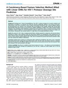
the AID362 is the dataset with the most features and samples. As for the second dataset of AID439 in bioassay, the performance of BFFA is very close to that of the ReliefF-BSTA. Although mRMR obtains the smallest d, its performance on Acc is not good. The following experiment over the dataset of AID721 in bioassay shows that the ReliefF-BSTA is the best of all and it selects less of the number of features. Although ReliefF gets the smallest d, its Acc is not desirable. As for the last dataset of AID1284 in bioassay, the BFFA has a similar performance with the ReliefF-BSTA. And the ReliefF-BSTA outperforms the rest methods. Fig. 11 depicts the iterative curves of the best solutions for all the datasets. In conclusion, the ReliefF-BSTA can better solve the feature selection problem in biomedical datasets. In this experiment, the Acc is used to represent the ability to discriminate between the active and inactive compounds. If the higher the Acc, then the more reliable the selected compounds and vice versa. Hence, from the results, we can see that the Relief-BSTA selects the most relevant compounds as far as possible on the basis of guaranteed reliability. This will make the HTS process easier and faster. 3) Discussion: As can be seen from the results, the ReliefFBSTA outperforms the other approaches in terms of the classification accuracy and the number of the selected features. The factors of the ReliefF-BSTA resulting better performance than the others are as follows. First, the information from the ReliefF is leveraged in the proposed method. Second, the proposed method maintains the solution diversity and algorithm convergence. Finally, the proposed method neatly solves the contradiction between the number of features and the classification accuracy.

V. C ONCLUSION In this paper, a simple but efficient hybrid feature selection method, named ReliefF-BSTA, is proposed to handle the feature selection problem for classification. The proposal combines a filter method ReliefF and a wrapper method BSTA as a hybrid one which works in two phases. In the first phase, the feature ranking and feature weights are calculated by using the ReliefF. In the second phase, the BSTA performs the search for a high quality solution. In addition, in our proposal, the initial solution of BSTA is generated based on the feature ranking. Therefore, the initial solution not only has some highly relevant features, but also is not easy to get into local optimum. A key characteristic of our proposal is that the new candidate is generated by the probability substitute operator based on feature weights. This operator can increase solution diversity. Moreover, a new selection strategy named relative dominance-based selection is proposed to compare two feature subsets. To analyze the performance of the proposed method, a battery of experiments have been conducted on seven wellknown datasets and a real biomedical case. However, it should be noted that the proposed method has not been applied to high-dimensional or online datasets. In the future, we expect to extend the proposed method for high-dimensional and online feature selection problems.

TABLE VII: Average results obtained by the seven algorithms Dataset

Bioassay AID362

Bioassay AID439

Bioassay AID721

Bioassay AID1284

Method

d

Acc(%)

S

Lasso

105

98.22

=

mRMR

99

98.19

=

ReliefF

69

98.25

=

SGA

71

98.22

=

BPSO

60.23

98.19

=

BFFA

61

98.55

=

ReliefF-BSTA

60

98.56

Lasso

55

69.64

-

mRMR

12

75.00

-

ReliefF

49

76.79

-

SGA

39

80.16

-

BPSO

37.50

80.16

-

BFFA

25.23

81.16

=

ReliefF-BSTA

23.53

82.01

Lasso

39

64.47

mRMR

49

57.89

-

ReliefF

8

80.26

-

SGA

41

80.14

-

BPSO

36.53

81.16

-

BFFA

36.23

82.09

-

ReliefF-BSTA

31.33

83.48

Lasso

68

76.55

-

mRMR

7

76.55

-

-

ReliefF

11

77.24

-

SGA

46

83.27

-

BPSO

40.07

84.28

=

BFFA

40.13

85.05

ReliefF-BSTA

38.50

85.25

ACKNOWLEDGMENT The authors thank the National Natural Science Foundation of China (Grant Nos. 61621062, 61873285, 61533020, 61533021, 61773405, 61725306), the 111 Project (Grant No. B17048), the Innovation-Driven Plan in Central South University (Grant No. 2018CX012), and Hunan Provincial Natural Science Foundation of China (Grant No. 2018JJ3683) for their funding support. R EFERENCES [1] J. Han, J. Pei, and M. Kamber, Data mining: concepts and techniques. 2011. [2] B. Xue, M. Zhang, W. N. Browne, and X. Yao, “A survey on evolutionary computation approaches to feature selection,” IEEE Transactions on Evolutionary Computation, vol. 20, no. 4, pp. 606–626, 2016. [3] G. A. Einicke, H. A. Sabti, D. V. Thiel, and M. Fernandez, “Maximumentropy-rate selection of features for classifying changes in knee and ankle dynamics during running,” IEEE Journal of Biomedical and Health Informatics, pp. 1–1, 2017. [4] S. Saha, A. K. Alok, and A. Ekbal, “Use of semisupervised clustering and feature-selection techniques for identification of co-expressed genes,” IEEE Journal of Biomedical and Health Informatics, vol. 20, pp. 1171–1177, July 2016.



AID362

90

80

98.5 Classification accuracy(%) # of selected features

98.4

70

98.3

60

98.2 0

10

20

30

40

50

60

70

80

90



98.6

50 100

Iterations AID439

40 Classification accuracy(%) # of selected features

82

30

80 0

10

20

30

40

50

60

70

80

90



84

20 100

Iterations AID721

86

46 44

82

42

80


40

78

38

76

36

74

34

72

32

70

30

68 0

10

20

30

40

50

60

70

80

90



84

28 100

Iterations AID1284

90

55

85

50

80

45

75

40

70 0

10

20

30

40

50

60

70

80

90




35 100

Iterations

Fig. 11: The Acc and d with respect to the number of iterations on AID362, AID439, AID721 and AID1284

[5] E. E. Bron, M. Smits, W. J. Niessen, and S. Klein, “Feature selection based on the svm weight vector for classification of dementia,” IEEE Journal of Biomedical and Health Informatics, vol. 19, pp. 1617–1626, Sept 2015. [6] C. Soguero-Ruiz, K. Hindberg, J. L. Rojo-lvarez, S. O. Skr?vseth, F. Godtliebsen, K. Mortensen, A. Revhaug, R. O. Lindsetmo, K. M. Augestad, and R. Jenssen, “Support vector feature selection for early detection of anastomosis leakage from bag-of-words in electronic health records,” IEEE Journal of Biomedical and Health Informatics, vol. 20, pp. 1404–1415, Sept 2016. [7] X. Liu, L. Ma, L. Song, Y. Zhao, X. Zhao, and C. Zhou, “Recognizing common ct imaging signs of lung diseases through a new feature selection method based on fisher criterion and genetic optimization,” IEEE Journal of Biomedical and Health Informatics, vol. 19, pp. 635– 647, March 2015. [8] J. W. Xu and K. Suzuki, “Max-auc feature selection in computer-aided detection of polyps in ct colonography,” IEEE Journal of Biomedical and Health Informatics, vol. 18, pp. 585–593, March 2014.

[9] A. Unler, A. Murat, and R. B. Chinnam, “mr2pso: A maximum relevance minimum redundancy feature selection method based on swarm intelligence for support vector machine classification,” Information Sciences, vol. 181, no. 20, pp. 4625 – 4641, 2011. Special Issue on Interpretable Fuzzy Systems. [10] L. Yu and H. Liu, “Efficient Feature Selection via Analysis of Relevance and Redundancy,” Journal of Machine Learning Research, vol. 5, pp. 1205–1224, 2004. [11] W. Shang, H. Huang, H. Zhu, Y. Lin, Y. Qu, and Z. Wang, “A novel feature selection algorithm for text categorization,” Expert Systems with Applications, vol. 33, no. 1, pp. 1 – 5, 2007. [12] M. F. Akay, “Support vector machines combined with feature selection for breast cancer diagnosis,” Expert Systems with Applications, vol. 36, no. 2, Part 2, pp. 3240 – 3247, 2009. [13] H. Peng, F. Long, and C. Ding, “Feature selection based on mutual information criteria of max-dependency, max-relevance, and minredundancy,” IEEE Transactions on Pattern Analysis and Machine Intelligence, vol. 27, pp. 1226–1238, Aug 2005. [14] I. Kononenko, “Estimating attributes: analysis and extensions of relief,” in European conference on machine learning, pp. 171–182, Springer, 1994. [15] M. Hall, Correlation-based feature selection for machine learning. PhD thesis, The University of Waikato, 1999. [16] A. W. Whitney, “A direct method of nonparametric measurement selection,” IEEE Transactions on Computers, vol. C-20, pp. 1100–1103, Sept 1971. [17] T. Marill and D. Green, “On the effectiveness of receptors in recognition systems,” IEEE Transactions on Information Theory, vol. 9, pp. 11–17, Jan 1963. [18] P. Pudil, J. Novovi?ov, and J. Kittler, “Floating search methods in feature selection,” Pattern Recognition Letters, vol. 15, no. 11, pp. 1119 – 1125, 1994. [19] I.-S. Oh, J.-S. Lee, and B.-R. Moon, “Hybrid genetic algorithms for feature selection,” IEEE Transactions on pattern analysis and machine intelligence, vol. 26, no. 11, pp. 1424–1437, 2004. [20] B. Tran, B. Xue, and M. Zhang, “Genetic programming for feature construction and selection in classification on high-dimensional data,” Memetic Computing, vol. 8, pp. 3–15, Mar 2016. [21] Y. Liu, G. Wang, H. Chen, H. Dong, X. Zhu, and S. Wang, “An improved particle swarm optimization for feature selection,” Journal of Bionic Engineering, vol. 8, no. 2, pp. 191 – 200, 2011. [22] S. Tabakhi and P. Moradi, “Relevanceredundancy feature selection based on ant colony optimization,” Pattern Recognition, vol. 48, no. 9, pp. 2798 – 2811, 2015. [23] A. Unler and A. Murat, “A discrete particle swarm optimization method for feature selection in binary classification problems,” European Journal of Operational Research, vol. 206, no. 3, pp. 528 – 539, 2010. [24] X. Zhou, C. Yang, and W. Gui, “State transition algorithm,” Journal of Industrial and Management Optimization, vol. 8, no. 4, pp. 1039–1056, 2012. [25] X. Zhou, C. Yang, and W. Gui, “Nonlinear system identification and control using state transition algorithm,” Applied mathematics and computation, vol. 226, pp. 169–179, 2014. [26] X. Zhou, D. Y. Gao, C. Yang, and W. Gui, “Discrete state transition algorithm for unconstrained integer optimization problems,” Neurocomputing, vol. 173, pp. 864–874, 2016. [27] X. Zhou, D. Y. Gao, and A. R. Simpson, “Optimal design of water distribution networks by a discrete state transition algorithm,” Engineering Optimization, vol. 48, no. 4, pp. 603–628, 2016. [28] M. Huang, X. Zhou, T. Huang, C. Yang, and W. Gui, “Dynamic optimization based on state transition algorithm for copper removal process,” Neural Computing and Applications, pp. 1–13, 2017. [29] F. Zhang, C. Yang, X. Zhou, and W. Gui, “Fractional-order pid controller tuning using continuous state transition algorithm,” Neural Computing and Applications, pp. 1–10, 2016. [30] J. Han, C. Yang, X. Zhou, and W. Gui, “Dynamic multi-objective optimization arising in iron precipitation of zinc hydrometallurgy,” Hydrometallurgy, vol. 173, pp. 134–148, 2017. [31] J. Han, C. Yang, X. Zhou, and W. Gui, “A new multi-threshold image segmentation approach using state transition algorithm,” Applied Mathematical Modelling, vol. 44, pp. 588–601, 2017. [32] X. Zhou, P. Shi, C.-C. Lim, C. Yang, and W. Gui, “A dynamic state transition algorithm with application to sensor network localization,” Neurocomputing, vol. 273, pp. 237 – 250, 2018. [33] Z. Huang, C. Yang, X. Zhou, and W. Gui, “A novel cognitively inspired state transition algorithm for solving the linear bi-level programming problem,” Cognitive Computation, May 2018.



[34] X. Zhou, C. Yang, and W. Gui, “A statistical study on parameter selection of operators in continuous state transition algorithm,” IEEE Transactions on Cybernetics, pp. 1–9, 2018. [35] X. Zhou, J. Zhou, C. Yang, and W. Gui, “Set-point tracking and multiobjective optimization-based pid control for the goethite process,” IEEE Access, vol. 6, pp. 36683–36698, 2018. [36] K. Kira and L. A. Rendell, “The feature selection problem: Traditional methods and a new algorithm,” in Proceedings of the Tenth National Conference on Artificial Intelligence, vol. 2, (San Jose, California), pp. 129–134, AAAI press, 1992. [37] A. Destrero, C. De Mol, F. Odone, and A. Verri, “A regularized framework for feature selection in face detection and authentication,” International Journal of Computer Vision, vol. 83, pp. 164–177, Jun 2009. [38] H. Peng, F. Long, and C. Ding, “Feature selection based on mutual information criteria of max-dependency, max-relevance, and minredundancy,” IEEE Transactions on Pattern Analysis and Machine Intelligence, vol. 27, pp. 1226–1238, Aug 2005. [39] L.-Y. Chuang, C.-S. Yang, K.-C. Wu, and C.-H. Yang, “Gene selection and classification using taguchi chaotic binary particle swarm optimization,” Expert Systems with Applications, vol. 38, no. 10, pp. 13367– 13377, 2011. [40] L. Zhang, L. Shan, and J. Wang, “Optimal feature selection using distance-based discrete firefly algorithm with mutual information criterion,” Neural Computing and Applications, vol. 28, no. 9, pp. 2795– 2808, 2017. [41] C. L. Blake and C. J. Merz, “Uci repository of machine learning databases [http://www. ics. uci. edu/˜ mlearn/mlrepository. html]. irvine, ca: University of california,” Department of Information and Computer Science, vol. 55, 1998.


A hybrid feature selection method based on binary state transition

A hybrid feature selection method based on binary state transition

Suggest Documents

A Hybrid Method of Unsupervised Feature Selection Based on Ranking

Hybrid Support Vector Machine based Feature Selection Method for

A proposed framework on hybrid feature selection

A Hybrid Feature Subset Selection Approach based on SVM ... - waset

A feature selection method based on an improved ... - SAGE Journals

A Feature Subset Selection Method Based On High ... - MDPI

Feature Selection Based Hybrid Anomaly ... - ScienceDirect.com

Feature Selection Based Hybrid Anomaly Intrusion ... - ScienceDirect

A hybrid feature selection method for credit scoring - EUDL

A Hybrid Method of Unsupervised Feature Selection ... - CiteSeerX

A Hybrid Feature Selection Method for Microarray Classification - IAENG

A Hybrid Feature Selection Method for Complex ... - IEEE Xplore

A Hybrid Gini PSO-SVM Feature Selection Based on Taguchi Method ...

Feature Selection Method Based on High-Resolution ...

Feature Selection Method Based on Artificial Bee Colony Algorithm ...

A Hybrid Approach for Effective Feature Selection

Stock Selection Based on a Hybrid Quantitative

Hybrid Feature Selection Method for Supervised ... - Springer Link

a genetic algorithm based wrapper feature selection method for ...

A New Entropy-based Feature Selection Method for Load Forecasting

A Knowledge-Based Feature Selection Method for ... - Semantic Scholar

A Consistency-Based Feature Selection Method ... - Semantic Scholar

A Filter Feature Selection Method for Clustering

ScienceDirect A Novel Feature Selection Method ...