Abstract. In this paper, we present a hybrid graph-drawing algorithm (GDA) for layouting large ... representation diagrams, logic trees, and networks. Other fields ...
arXiv:1507.02766v1 [cs.GR] 10 Jul 2015
A Hybrid Graph-drawing Algorithm for Large, Naturally-clustered, Disconnected Graphs Toni-Jan Keith P. Monserrat, Jaderick P. Pabico and Eliezer A. Albacea
Abstract In this paper, we present a hybrid graph-drawing algorithm (GDA) for layouting large, naturally-clustered, disconnected graphs. We called it a hybrid algorithm because it is an implementation of a series of already known graph-drawing and graphtheoretic procedures. We remedy in this hybrid the problematic nature of the current force-based GDA which has the inability to scale to large, naturally-clustered, and disconnected graphs. These kinds of graph usually model the complex inter-relationships among entities in social, biological, natural, and artificial networks. Obviously, the hybrid runs longer than the current GDAs. By using two extreme cases of graphs as inputs, we present in this paper the derivation of the time complexity of the hybrid which we found to be O(|V|3 ).
1. Introduction Information that abstractly describes the inter-relation-ships among entities in most complex systems is mathematically represented using graphs. Graphs as tools are an intuitive approach for visualizing entities because they make it easier for humans to understand the relationships between different entities. Because of this, graph visualizations of entities, as well as that of processed data, are used in many types of applications. For example, computer science concepts are usually easier to understand with the use of visualization concepts such as data flow diagrams, subroutine-call graphs, program nesting trees, object-oriented class hierarchies, entity-relationship diagrams, organization charts, circuit schematics, knowledgerepresentation diagrams, logic trees, and networks. Other fields of sciences also use graph visualization to represent information like concept lattices, evolutionary trees, molecular drawings, and maps and map schematics [1]. Because of the utility of graph visualization for viewing data that can be understood by the user in a vast number of applications, many techniques were devised for drawing graphs efficiently and beautifully. Since the first paper by Knuth in 1963 on drawing flowcharts for visualization purposes [1, 2], there are now about 300 existing algorithms on graph drawing
1
itself, some of these have improved the existing ones by utilizing the research advances made in topological and geometrical graph theory, graph algorithms, data structures, computational geometry, visual languages, graphical user interfaces and software visualization [1]. However, given the numerous available algorithms, there is no one-size-fits-all graph drawing algorithm for any given graph. It is also important to identify the class to which a certain graph belongs. This is because several graph-drawing algorithms can only make effective visualizations on certain graph classes. Additionally, there are several approaches that exist in drawing graphs. Some of these approaches are drawing conventions, aesthetics, constraints and efficiency. These approaches include topology-shape-metrics, hierarchical, visibility, augmentation, divide and conquer, and force-directed. In the current effort, we developed a hybrid force-directed approach algorithm based on the one developed by Kamada and Kawai [3]. Here, we used a clustering algorithm called Markov cluster algorithm to cluster the original vertices into sub-graphs. We then used the original Kamada-Kawai (KK) force-directed algorithm to draw the vertices in each sub-graph. We considered each sub-graph as a big “phantom” vertex and applied the Iterative KamadaKawai (IKK) algorithm to draw the respective locations of the non-uniform-sized phantom vertices. In this paper, we analyze the runtime of our hybrid graph drawing algorithm (HGDA). We illustrate our derivation by considering input graphs in extreme cases: a fully connected graph Ga (Va , Ea ) and a graph with no edges Gb (Vb , ∅). With these input graphs, we found out that HGDA has O(|V|3) runtime complexity.
2. Review Because graph drawings are used primarily to visualize information in a more understandable way, there are certain criteria that should be met when doing it. Drawing graphs should obviously include the type and properties of the graph to be drawn. This is important because several graph drawing algorithms are only designed to efficiently work on certain types of graphs. It is also essential to know that there is no optimum drawing for any graph because human perception changes from every individual. It should be noted that although the product of a graph-drawing algorithm may be subjective, it also has objective criteria such as drawing convention, aesthetic and constraints. For a graph drawing to be admissible, it has to have some drawing conventions that it should follow. Examples of these conventions are having polyline for edges, using planar mathematics for layouting, and using grids to locate the vertices. A certain type of convention that is often used in graph drawing theories [1] is the straight-line drawing. To objectively evaluate the aesthetics of a graph drawing, it specifies graphic properties of drawing that can achieve readability at the least. Some common aesthetic evaluation includes minimization of the total number of crossings between edges and minimization of the drawing area. These two efficiently use the drawing space without sacrificing the readability of the relationship between vertices [4–6]. Additionally, constraints must also be considered specifically when drawing sub-graphs. Creating certain constraints on position and space provides how each subgraph should be drawn. Example of a common constraint would have a given vertex be
2
drawn at the center of the drawing area. Another one is to have some of vertices be clustered or enclosed within a predefined shape [7, 8]. Because of these criteria, several approaches in graph drawing were established. One of these approaches is through the use of force-directed algorithms (FDA). Due to their flexibility, ease of implementation and often-pleasant drawings, FDA are often used and improved [9]. Conventionally, FDA use straight-line drawings to draw edges in undirected graphs. FDA simulate some “force” that is directed to each vertex. When the minimal energy of the whole system is already achieved, the position of the vertices in the graph are said to be in its balanced state. To find the balanced state of the graph, FDA incorporate two main functions: (1) The force model that simulates the forces acting on each of the vertex; and (2) An iterative algorithm to find the local minimal energy configuration [1]. The KK algorithm takes in a connected graph G(V, E) and uses the graph theoretic distance (GTD) between each pair of vertices u ∈ V and v ∈ V as its force model. GTD between vertices u and v is calculated as the number of edges on a shortest path from vertex u to vertex v. Usually, the aim of the FDA that uses GTD as a force model is to find the Euclidean distance between u and v to be approximately proportional to their GTD. KK includes an energy or spring view in the GTD [1, 3]. Because of this, KK was able to create symmetric drawings with relatively few edge crossings, which is practically similar to drawing isomorphic graphs [3]. It should be noted, however, that KK only focused on fairly simple graphs. Originally, it was intended to solve undirected, non-weighted, simple and fully connected graphs [10]. An obvious problem for KK is the its inability to scale to handle large graphs. This inability is common also for other FDA. FADE [9], a fast algorithm for two-dimensional drawing of large undirected graphs, was one of the more successful implementations of FDA that scale to larger graphs. It uses clustering before applying FDA, although primarily to lessen the computational time, and secondarily for maintaining the visualization better [9]. There are many ways to cluster large graphs into manageable sub-graphs. Examples of these are the graph theoretic clustering [11] and the geometric clustering [12] procedures like the ones being used in FADE, and the Markov Cluster Algorithm (MCL) [13]. One of the advantages of MCL is that it does not have any high level procedural rules for splitting or joining groups. The idea of MCL is to simulate a system of “current” C flowing inside the graph, promote that system when C is strong, or demote the system when C is weak. The computational paradigm is that C between natural groups in the graph will wither away, revealing the cluster or sub-graph [13]. Clustering a graph into sub-graphs defines the structure and natural clusters within the graph. By doing so, it arranges the vertices in the adjacency matrix A by creating blocks of “1s” diagonally in A where the clusters are formed. This makes it easy for the FDA to find the equilibrium by re-ordering the vertices according to their connections within and between the clusters, as opposed to the original procedure of randomly arranging vertices in G [14].
3
3. Theoretical Framework 3.1. Preliminary A graph G is a pair of sets (V, E). V is the set of vertices and the number of vertices n = |V| is the order of the graph. The set E contains the edges of the graph. In an undirected graph, each edge is an unordered pair {v, w}. A vertex w is adjacent to a vertex v if and only if (v, w) is an element of the set E. In an undirected graph, the abstract relationship represented by (v, w) is the same as that of (w, v). A path in a graph is a sequence of vertices w1 , w2 , . . . , wn such that there exists an edge (wi , wi+1 ) where 1 ≤ i < n. The length of the path is equal to number of edges (n − 1), where n = |V| is the number of vertices that runs along that selected path. A simple path is a path such that all vertices are distinct, with the exception of the first and last vertex of the path, which can be the same vertex [15]. A graph G′ (V ′ , E ′ ) is a sub-graph of G(V, E) if V ′ ⊂ V and E ′ ⊂ E (V ′ × V). T
A graph G(V, E) with n = |V| vertices can be described by an n × n adjacency matrix A whose rows and columns correspond to vertices. The matrix elements Au,v = 1 if (u, v) is part of E. Au,v = 0 otherwise. A graph is connected if there is a path between u and v for each pair of vertices u and v.
3.2. Clustered and disconnected graphs Graphs that are of small-world, scale-free characteristics are naturally clustered with some disconnected components. Small-world graphs are characterized by a very small network diameter, which usually values within six for naturally-occurring social networks SN [16, 17]. The degree ∆i of a vertex vi counts the number of incident edges of vi . A symmetric matrix Ai,j represents an undirected graph G, where Ai,j = Aj,i = 1 if vi is incident to vj . P Thus, ∆i = nj=1 Ai,j . For most SN , the frequency distribution ρ(∆) of the degree in G has been found by various researchers [18–20] to asymptotically follow the power law distribution of the form ρ(∆) = α × ∆ϕ . For social networks, and all other biological networks, the power usually takes the value −3 ≤ ϕ ≤ −2. Having ρ(∆) ∼ α × ∆ϕ makes SN scale-free [18]. Figure 1 shows an example of a small-world, scale-free graph that is naturally clustered and disconnected.
3.3. Connected components The connected components of an undirected graph G are the maximal disjoint sets V1 , V2 , . . . , Vn such that V = V1 ∪ V2 ∪ · · · ∪ Vn , and the vertices u, v ∈ Vi if and only if u is reachable from v and v is reachable from u [22, 23]. Two methods are generally used to identify the connected components of G: (1) The breadth-first-search (BFS); and (2) The depth-first-search (DFS). We can use any of these two to see if a certain path from u to v exists for each vertex pair of (u, v) [24]. Given a starting vertex v0 , BFS systematically 4
Figure 1: An example large, naturally-clustered and disconnected graph G drawn using KK. This graph is based on the co-authorship network of Filipino computer scientists created by Pabico [21] with |V| = 605. Notice that there exist some pronounced vertex clusterings in each connected component. search a given graph of vertices that has a path from v0 . First, BFS lists all vertices that are adjacent to v0 . Then, it starts again with another vertex vi in the list that is directly connected with the previous vertex. The usual convention is to take the first vertex in the list as the vi . BFS again does the listing of vertices that are directly connected to vi . The algorithm stops when there are no more vertices that have a path from v0 . Now, if there still exist vertices that are not listed after the BFS has been done, then the said graph is considered disconnected. The complexity of a BFS algorithm that returns all connected components is 0(|V| × |E|). In DFS, the traversal is done in a depth-first fashion, wherein the outcome is a forest of depthfirst trees. Each tree in the forest contains vertices that belong to a different subgraph. The correctness of DFS as a test for graph connectivity follows directly from the definition of a spanning tree, and from the fact that the graph is undirected. This means that a depth-first tree is also a spanning tree of a graph induced by the set of vertices in the depth-first tree. Assuming that the graph is stored using a sparse representation, the run time of the DFS is θ(|E|).
3.4. MCL The MCL starts from a random starting vertex v0 ∈ G and walks to other vertices connected to v0 . Here, G maybe described using a similarity matrix. The traversal usually does not leave the graph’s cluster until many of the cluster’s vertices have been visited. The idea of the algorithm is that it simulates “flow” within a graph. The flow is done iteratively wherein after each step, MCL demotes the edges within the distant nodes and promotes the edges of the nearby nodes. To do this, MCL takes the corresponding n × n adjacency matrix A of the graph G and normalizes each column to obtain a stochastic matrix M. This includes adding the diagonal elements in the adjacency matrix to include self-loops for all nodes. After initializing the matrix, the algorithm uses two alternating functions: (1) expansion, which is used to flatten the stochastic distributions in the columns and causes the edges 5
and paths of the random walker to become evenly spread; and (2) inflation, which contracts them to favor paths. It is said that the MCL algorithm’s complexity is O(n3 ), where n = |V| is the number of vertices of the input graph. This is the same as the cost of multiplying two matrices of dimension n. It is also noted that the inflation step of the algorithm has a complexity of O(n2 ). The mathematical analysis on the time complexity of MCL is discussed in detail by van Dongen [13].
3.5. Kamada-Kawai The KK algorithm [3] is commonly described as a “spring-embedder” where the vertices v1 , v2 , . . . , vn ∈ V are considered particles that are mutually connected by springs in a dynamic system. Each vertex vi ∈ V is initially located within the canvass with its twodimensional coordinates (xi , yi ). The human-readable layout of vertices in the canvass is directly related to the dynamic balance of the energy E in the spring system. In other words, E is modeled as a system of springs with a degree of elasticity wherein a desired resting length is achieved when the system reaches an equilibrium. This physical fact is described mathematically in Equation 1. The best layout for a given graph G is at minimum E.
E =
n X X 1 n−1 kij (Di,j − L × dij )2 2 i=1 j=i+1
L0 maxi