A Hybrid Graph Model for Unsupervised Object ... - CiteSeerX

A Hybrid Graph Model for Unsupervised Object Segmentation Guangcan Liu1 Zhouchen Lin2 1 Shanghai Jiao Tong University, China 1

{roth,yyu}@apex.sjtu.edu.cn

2

Xiaoou Tang2 Yong Yu1 2 Microsoft Research Asia {zhoulin,xitang}@microsoft.com

Abstract In this work, we address the problem of performing class specific unsupervised object segmentation, i.e., automatic segmentation without annotated training images. We propose a hybrid graph model (HGM) to integrate recognition and segmentation into a unified process. The vertices of a hybrid graph represent the entities associated to the object class or local image features. The vertices are connected by directed edges and/or undirected ones, which represent the dependence between the shape priors of the class (for recognition) and the similarity between the color/texture priors within an image (for segmentation), respectively. By simultaneously considering the Markov chain formed by the directed subgraph and the minimal cut of the undirected subgraph, the likelihood that the vertices belong to the underlying class can be computed. Given a set of images each containing objects of the same class, our HGM based method automatically identifies in each image the area that the objects occupy. Experiments on 14 sets of images show promising results.

1. Introduction Object segmentation is one of the fundamental problems in computer vision. Its goal is to segment an image into foreground and background, with the foreground solely containing object(s) of a class (Figure 1). There are two categories of algorithms: supervised and unsupervised. Supervised algorithms require either manually segmented masks in training images [10, 18, 22], specify shape templates [7, 14, 18, 23, 24], or other kinds of priors (e.g., object part configuration [21] or class fragments [4]). These algorithms may be applicable to a particular object class [23], a range of objects [14, 22], or object classes [4, 7, 10, 18, 21, 24] provided that the class dependent priors are available. However, as a practical object recognition system needs to handle a large number of classes of objects and most classes may require many training samples due to significant intraclass shape and appearance variances, it is important that the learning does not involve any human interaction. This

978-1-4244-1631-8/07/$25.00 ©2007 IEEE

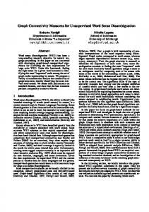
Figure 1. Our HGM based object segmentation. Inputs: A set of images each consisting of objects (foreground) of a class and different backgrounds. Outputs: Regions solely containing objects of the class. The whole process is fully automatic.

makes unsupervised algorithms more appealing. There has been sparse research in this direction. Borenstein and Ullman [5] used the overlap between automatically extracted object parts (or fragments) to determine the foreground and the background. As individual parts are considered independently, the approach is prone to wrongly judge background clutters as foreground parts. Winn and Jojic [19] combined all images together to find a consistent segmentation based on the assumption that the object shape and color distribution pattern are consistent within class and that the color/texture variability within a single object of a class is limited. Moreover, each image should only contain one object of the class. Rother et al. [16] showed that it is possible to use only two images to segment their common parts simultaneously. They required the common parts to have similar shape and color/texture. Russell et al. [17] segmented images in multiple ways and then borrowed techniques from document analysis to discover multiple object classes. Their assumption was that some regions in some of the segmentations are correct for each object. As segmentation precedes class discovery, it is usually hard to have accurate segmentation. Due to the limitations of these existing methods, we aim at proposing a novel unsupervised algorithm that can produce more accurate object boundaries for images of objects of the same class, where the assumption on the variance of object shape and color/texture is much weaker and images can contain multiple objects. To ensure robustness, we follow the doctrine that object segmentation should be handled in parallel to object recognition [10, 11, 18, 19, 21, 24] as they are strongly coupled problems. Although no annotated training images are avail-

able, as long as there are enough images, the common patterns of the object class will appear frequently and the effect of the background will fade out as it is much less structured compared to the objects. So our target is to segment a large number of images simultaneously. As we will not assume small intra-class shape variance (e.g., Figure 1(a)), unlike [10, 18, 24], we do not expect that there will be a global shape prior for recognition. Therefore, we adopt local shape priors based on the work of Agarwal and Roth [2]. We first extract the object parts using an interest points detector [9]. The object parts and the weak spatial relationship among them form our shape priors. The local shape priors provide very weak top-down constraint on the object shape, as the object parts are only sparsely distributed across the objects, and very often they also reside in the background. On the other hand, like [11], we also oversegment the images into superpixels [13] and group homogeneous superpixels into relatively large subregions [20]. The image-based grouping operators also provide a very weak bottom-up constraint on the object shape. To combine the top-down and the bottomup information and bridge the gap between them, we propose a hybrid graph model (HGM, Figure 2) that describes the relationship among the object parts and the superpixels. The vertices of a hybrid graph represent the entities associated to the object class or local image features, e.g., object parts and superpixels. The vertices are connected by directed edges and/or undirected ones. A directed edge represents the dependence between the entities that it connects (for recognition), while an undirected edge represents the similarity between the entities (for segmentation). The likelihood that the entities belong to the underlying class can be computed by solving an optimization problem that merges a random walk on the directed subgraph and the minimal cut of the undirected subgraph. Using the HGM, we can integrate the recognition and the segmentation in a unified framework and form a global decision on the boundaries of objects. Compared to the previous unsupervised algorithms [5, 16, 19, 17], the main advantages of our HGM based method are: - Larger variation in shape (including position, size, pose, and profile) is allowed within a class. - Larger variation in color/texture is allowed not only within class but also within object. - Multiple objects of the same class are allowed in each image. - More accurate output of object boundaries. The remainder of this paper is organized as follows. Section 2 introduces the general formulation of a hybrid graph model. Section 3 details our HGM based object segmentation approach. Section 4 presents an optional algorithm

Figure 2. An illustration of the hybrid graph. A vertex denotes an entity in reality. A directed edge represents the relation of conditional dependence between a pair of entities. An undirected edge represents the relation of homogeneous association between a pair of entities. Between each pair of vertices, there are at most three edges: two directed edges and one undirected edge. In some scenarios, it is possible that some vertices are isolated.

for performance improvement. Section 5 shows the experiments and results. And Section 6 concludes this paper.

2. The Hybrid Graph Model 2.1. The Hybrid Graph From previous observations, we need to model the relationship between shape and color/texture at the same time. There are two types of relationship among the entities:
Conditional Dependence The conditional dependence represents the relation of the occurrence of one entity being dependent on the occurrence of the other. It is directed and asymmetric. In our object segmentation task, it represents the concurrence of the object parts.
Homogeneous Association The homogenous association usually measures the “similarity” among entities. It is undirected and symmetric. In our case, it represents the color/texture similarity and the spatial adjacency among superpixels. Let V = {v1 , · · · , vn } be n entities. Then by considering the above two types of relationship, we have two matrices: 1. Conditional Dependence Matrix P : P = [pij ]n×n , where pij measures the conditional dependence of vi on vj . 2. Homogeneous Association Matrix A: A = [aij ]n×n , where aij measures the homogeneity between vi and vj . Therefore, a general hybrid graph (Figure 2) G = (V, E) consists of a finite vertex set V and an edge set E with each

edge connecting a pair of vertices. The weights assigned to directed edges and undirected ones correspond to matrix P and matrix A, respectively.

2.2. Computing the Likelihood Using the HGM Given the relationship among the entities, it is possible to infer the likelihood of each entity belonging to the object. Suppose each vertex i is associated with a likelihood πi . From the directed component of the hybrid graph, if vj depends on vi , we may expect that vi is more important than vj and vi is more likely to belong to the object. Hence, the interdependence among the entities forms a Markov Chain with the transition matrix P . Ideally, like PageRank [6], this → results in a stationary distribution − π = (π1 , ..., πn )T of P that assigns each entity a likelihood: → − → π TP = − π T. (1) On the other hand, from the undirected component of the hybrid graph, if two entities vi and vj are strongly associated, they are more likely to belong to the object or background simultaneously. So the segmentation should minimize the cut cost
aij (πi − πj )2 . (2) i,j

Putting the above two criteria together, we have an opti→ mization problem to calculate the likelihood vector − π:
→ → π −− π ||2 + α min ||P T − aij (πi − πj )2 , (3) i,j

→ → subject to− π T− π = 1, where α is a positive parameter used to balance the effects of the two criteria. In our experiments, we fix α = 1. The solution to problem (3) is the eigenvector associated to the minimum eigenvalue of the following matrix: (I − P )(I − P T ) + αLA ,

(4)

where LA is the Laplacian matrix of the undirectedcomponent:  LA = DA − A with DA = n n diag{ j=1 a1j , · · · , j=1 anj }, and I is the identity matrix.

Figure 3. Illustration of HGM based segmentation. Given an image (1), a mask map (4) has to be learnt. To this end, we obtain object parts (2.1) using the Harris interest point detector and group the pixels into superpixels (2.2). Then we further cluster object parts and superpixels into visual words (2.3) and mid-level oversegmentation (2.4), respectively. Next, we incorporate the acquired priors into an HGM by defining the conditional dependence matrix P according to shape priors and the homogenous association matrix A according to the color/texture priors. With the mask map (4) computed from the HGM, the image can be easily segmented (5).

3.1.1

Acquiring Local Shape Priors

3. HGM Based Object Segmentation Our HGM based object segmentation algorithm is outlined in Figure 3. In the following, we describe details of each step.

3.1. Acquiring Prior Information We first resize all images to about the same size, with the longer side being 320 pixels. Then the remaining preprocessing procedure mainly aims at acquiring the prior information of the object class.

Our local shape priors consist of visual words [17] and the spatial distances between them. A visual word is the center of a cluster of local windows that have similar appearance. It represents the whole cluster and is a feature of local appearance of an object class (e.g., the tyres of cars). The aforementioned “object part” is an instance of the cluster that a visual word represents. 1. Building the Codebook We follow the methods in [2, 10]. Firstly, a number of images are randomly chosen from all provided images and

are converted to grayscale. These images are considered as “special” self-training images for extracting the shape priors of the class. Secondly, object parts with rich textures are detected by extracting windows of size 25 × 25 around the points detected with the Harris interest point detector [9] (Figure 3(2.1)). Thirdly, all detected parts are clustered into several clusters by agglomerative clustering [10] (Figure 3(2.3)). All the cluster centers form the visual words that describe the local appearances of the class. The codebook consists of all the visual words. It can be refined by HGM for higher accuracy. We defer the details until Section 4. 2. Building the Spatial Relation Table As we are to address larger shape variation, unlike deformable templates [7, 14, 18, 23, 24] and implicit shape model [10], we can only assume very weak shape configurations. We hence only consider the spatial distance between visual words. By iterating over all selected images and matching visual words to every detected object parts using NGC (Normalized Grayscale Correlation) measure [10], we have a table of the spatial relation between pairs of visual words: [vwi , vwj , dij ∼ N (µij , σij )],

(5)

where vwi and vwj are two visual words and N (µij , σij ) is a Gaussian that fits the distribution of the spatial distance dij between object parts matched to vwi and vwj . Unlike [2], which also considered direction between object parts, we ignore the direction because we allow arbitrary object orientation. 3.1.2

Acquiring Color/Texture Priors

Color and texture are also features of objects. As object regions should consist of subregions that are homogeneous in color or texture, for computational efficiency, we shall not consider pixel level segmentation. So we first oversegment the images into superpixels [13] (Figure 3(2.2)) then use the mid-level clustering algorithm proposed in [20] to group the superpixels into much larger subregions (Figure 3(2.4)). Then the similarity between superpixels can be measured by whether they belong to the same subregions. Using midlevel clustering results as the similarity measure is superior to directly using pairwise similarities as in [15], because the clustering algorithm in [20] incorporates more information to judge the homogeneity of a subregion.

3.2. Learning Mask Maps via HGM Given an image, we aim at learning a mask map that gives each superpixel a probability of lying inside object(s). Our basic notion is to integrate all the priors into a unified framework. However, there is difficulty in directly applying shape priors to superpixels and color/texture priors to object

parts, because object parts are square while superpixels are irregular. With HGM, we can overcome this difficulty. 3.2.1

The Hybrid Graph for Object Segmentation

Our hybrid graph G = {V, E} for object segmentation (Figure 3(3)) has two types of vertices: V = Vp ∪ Vs , where Vp is the set of vertices representing object parts and Vs denotes superpixels. The vertices in Vp are mainly connected by directed edges and those in Vs are connected by undirected ones. Initially, the shape priors are applied to object parts, and color/texture priors are applied to superpixels. In order to make these two different priors interact with each other, vertices in Vp can not only connect to each other but also connect to those in Vs by undirected edges. In such a manner, via the extra undirected edges, shape priors can also act on superpixels and color/texture priors can also act on object parts as well. Then the learning process is achieved by coupling two different subsystems: a recognition system represented by the directed subgraph playing the role of finding the object parts belonging to the object(s) and a segmentation system represented by the undirected subgraph that is responsible of grouping superpixels. The two subsystems are coupled by the extra undirected edges. Next, we have to define the conditional dependence matrix P and the homogeneous association matrix A. 3.2.2

Defining Conditional Dependence Matrix P

In the following, we cast the recognition procedure into the HGM via defining the conditional dependence matrix P according to the spatial configuration among the object parts detected in an image. In the HGM, a vertex vi ∈ Vp denotes an object part Oi , observed at location i . Let ei be the event of [Oi , i ] being observed. For an object class C, we intend to estimate the likelihood of each object part lying inside the object(s) of C. The likelihood can be measured by the following conditional probability: πi = P (ei |C). As no annotated images are available, it is not easy to define the object class C explicitly. So directly calculating the likelihood is difficult. We therefore regard πi ’s as latent variables and try indirectly calculating it as follows:
πj = P (ej |C) = P (ei |C)P (ej |ei , C) i
=j

=




πi P (ej |ei , C).

i
=j

Comparing the above equation with equation (1) reveals that pij should be defined as the conditional dependence of ej on ei , i.e., pij = P (ej |ei , C). With the event ei fixed, ej

is equivalent to a new event e˜ ij = [Oi , Oj , dij ] that Oj is observed at the location with distance dij from Oi . Hence = P (ej |ei , C) ∝ P (˜eij |C).

pij

To compute pij , we have to estimate P (˜eij |C). By matching Oi and Oj to the codebook of the object class C, we obtain a set of interpretations Iij = {Ii
j
|Ii
j
is the event that Oi and Oj are matched to the visual words vwi
and vwj
, respectively} (i.e., Oi and Oj are interpreted as the visual words vwi
and vwj
, respectively). Then
P (˜eij |C) = P (Ii
j
|C)P (˜eij |Ii
j
, C) Ii
j
∈Iij

=




P (Ii
j
|C)P ([vwi
, vwj
, dij ]|Ii
j
, C),

Ii
j
∈Iij

where P (Ii
j
|C) can be computed as |I1ij | , assuming the independence on C and the equal probability of each event, and P ([vw  i
, vwj
, dij]|Ii
j
, C) can be computed as √

1 2πσi
j


exp −

(dij −µi
j
)2 2σi2
j


due to equation (5).

As mentioned, the shape priors cannot be directly applied to superpixels. So the matrix P is only defined on the vertices of object parts. To be precise, the matrix P is defined as the following:  P (˜eij |C) , if vi ∈ Vp , vj ∈ Vp , i = j, eik |C) k P (˜ pij = 0, otherwise. 3.2.3

Defining Homogeneous Association Matrix A

Homogeneous association is defined on both object parts and superpixels. We expect that spatially close entities have similar likelihood, and object parts should act on nearby superpixels and vice versa. Therefore, the weights are defined differently according to the types of the vertices:   exp(−κ1 d2ij ) + sij , if vi ∈ Vs , vj ∈ Vs , exp(−κ2 dij ), if vi ∈ Vp , vj ∈ Vs , (6) aij =  exp(−κ1 d2ij ), if vi ∈ Vp , vj ∈ Vp ,   1, if vi and vj are in the same subregion, where sij =  0, otherwise, where dij is the spatial distance between the entities (object parts or superpixels), and in our experiments κ1 and κ2 are chosen as 0.04 and 0.2, respectively. The extra sij here further encourages the superpixels belonging to the same subregion (Figure 3(2.4)) to have similar probability. 3.2.4

Obtaining Mask Maps and Segmentation Results

By solving the minimum eigenvalue problem described in Section 2.2, we obtain a likelihood vector giving every object part and superpixel the probability of lying inside desired object. In this work, the segmentation task only needs

the probability of superpixels. However, as mentioned, the calculation for that of object parts cannot be waived, because object parts carry shape priors that cannot be modelled by superpixels. Given a mask map (Figure 3(4)), where the intensities have been normalized to between 0 and 1, the mask map is firstly segmented into a few regions by agglomerative clustering: the two nearby regions having the closest intensities are merged, as long as the difference between their intensities stays below a certain threshold 0.03. To arrive at the final segmentation result (Figure 3(5)), we next select a threshold t using Otsu’s discriminant analysis [8]. At last, we adopt a greedy region growing based method: beginning with the regions with the intensities greater than (1 + t)/2, merge the next adjacent region with the highest intensity until all the intensities of adjacent regions fall below t.

4. Improving Performance by Refining the Codebook The goal of constructing a codebook is to select important features that well describe the local appearance of an object class. However, interest point detectors alone are not enough to select good features because they just consider the local information in a single image. The accuracy of codebook can be improved by our HGM. Given n object parts {O1 , · · · , On } extracted from images and their clustering result {C1 , · · · , Cm }, instead of using all the clusters as visual words to construct the codebook, we aim at selecting k (k < m) clusters that are “important” to an object class. The importance of a cluster can be computed from the importance of the object parts that belong to it. To this end, we design a hybrid graph G to calculate a likelihood (or → score) vector − π , with each πi giving an object part Oi the “probability” of being important. Its vertices are the object parts. In the following, we define the matrices P and A. Let Oi be the event that the object part Oi is important. Following the similar argument in Section 3.2.2, we have that the entry pij of the conditional dependence matrix P should be in the form: pij = P (Oj |Oi ), which is the probability of an object part Oj being important, given that another object part Oi is important. To appropriately define P (Oj |Oi ), we propose the following two principles: 1. If an object part is important, then the object parts similar to it should also be important, i.e., P (Oj |Oi ) ∝ Sim(Oj , Oi ). 2. If an object part is distinctive, it should be important, i.e., P (Oj |Oi ) ∝ dst(Oj ).

In this work, we use the Euclidean distance dg (Oi , Oj ) between their grayscale vectors to measure the similarity between Oi and Oj . The distinctiveness of an object part is defined according to a heuristic notion: an object part is distinctive if there is another object part which is close to it in space, but far away from it in texture. Therefore, the distinctiveness of the part Oj can be computed as: dst(Oj ) = max dg (O, Oj )/ds (O, Oj ), O

where O is another object part that is detected in the same image with Oj and ds (O, Oj ) is the spatial distance between O and Oj . Summing up, we may make P (Oj |Oi ) proportional to p˜ij , where p˜ij = exp(−λdg (Oi , Oj )/dst(Oj )), in which λ = 0.2 is a parameter. Consequently, pij is defined as  pij = p˜ij / j
p˜ij
by normalizing the probability to 1. With this definition, an object part will have a high importance score if there are many other object parts similar to it and it is distinctive itself. On the other hand, the homogeneous association matrix A is defined to encourage that the object parts belonging to the same cluster to have a close score: 1, if Oi and Oj belong to the same cluster, aij = 0, otherwise. By solving the minimum eigenvalue problem in Section 2.2, we have the importance of each part. Then for a cluster Ci , its importance is computed according to the scores of its member object parts:
Imp(Ci ) = |Ci | πj , Oj ∈Ci

where |Ci | is the number of parts belonging to Ci and πj is the importance of part Oj . Note that we favor clusters with wide coverage (more member parts) by multiplying the sum of scores with |Ci |. Then the clusters are sorted in descending order of their importance, and we select the top k (k = 30) clusters with positive importance scores to construct the codebook. In the experiments, we find that this approach can make the segmentation more accurate.

5. Experimental Results We apply HGM to 12 public image sets with 3200 images in total: ten image sets with 1300 images are from Corel photo CDs [1], and the other two sets (Airplane and

object class Airplane Antique Bus Cat Dinosaur Dog Eagle Leopard Motorbike Old Car Owl Plane Average

# of images total special 1074 200 100 60 100 60 100 60 100 60 200 60 100 60 100 60 826 100 200 60 100 60 200 60 – –

performance recall precision 0.8060 0.7638 0.7661 0.8073 0.8597 0.8056 0.7168 0.8019 0.9785 0.9074 0.7291 0.6819 0.8760 0.8059 0.7587 0.7045 0.8526 0.8289 0.8096 0.7432 0.9068 0.8184 0.8516 0.7947 0.8240 0.7866

Table 1. Evaluation results on 12 object classes. “# special images” refers to the number of “special” self-training images for extracting the shape prior (Section 3.1.1).

Motorbike) with 1900 images are from Caltech [12] (Table 1). Each set consists of a number of images each containing objects of the same class in a variety of positions, sizes, poses, and profiles. After tweeking on the Bird image set of Corel 1 , we fix the parameters and apply them to all experiments which are of totally different object classes. Our system automatically outputs the foreground of the images. The numbers of “special” self-training images (Section 3.1.1) for each object class are also listed in Table 1. Figure 4 shows some examples of segmentation results. We only present five examples for each class due to the page limit. To give a quantitative evaluation of our approach, we acquire ground truth masks manually. Let A be the ground truth mask, and B be the mask output by our system. We define recall and precision as follows: recall = |A ∩ B|/|A|,

precision = |A ∩ B|/|B|, (7)

where |.| denotes the area of a region. Recall and precision are two competitive measurements. It is very easy to make only one of them high, but the segmentation is good only when both of them are high. Table 1 shows the evaluation results on all the 12 image sets, where for each object class all the images are used to compute those values because the whole segmentation process is fully automatic. One can see that the performance of HGM is quite satisfactory. That the performance varies on different data sets is due to our assumption: similar non-class clutters should not appear frequently in the images. Otherwise, our system will judge them to be part of the object (e.g., the shadow of cars will be judged as part of the cars. And please also refer to the second row of Figure 4, where the labels are always 1 Parameter selection is unavoidable, as in those unsupervised algorithms [5, 16, 17, 19].

Figure 4. Some examples of segmentation results of the 12 object classes. Each row is of the same class.

beside the antiques.). Without additional class specific information, such errors are hard to be corrected. Comparison Results We also apply HGM to two object classes (side view of Cars and Horses) that have been used by LOCUS [19]2 . The shape variation within class and/or color/texture variation within object in these two image sets are smaller than those in the sets we have just presented above. We use the same evaluation metric “accuracy” defined in [19] to measure the performance of HGM: “accuracy” = (|CLF | + |CLB |)/|Image|,

(8)

2 As listed in the introduction, we are only aware of four papers on unsupervised object segmentation [5, 16, 17, 19]. However, [16] and [17] actually address slightly different problems from ours. So we mainly focus on comparing with LOCUS [19], which was claimed to be more accurate than [5].

where CLF and CLB are the correctly labelled foreground and background pixels, respectively, and Image is the whole image. Note that their “accuracy” is a different measure from our recall and precision defined in equation (7). For comparison, we quote results from Borenstein et al. [3] which requires 54 hand segmented training data for the Horse image set, and LOCUS [19] which is also an unsupervised object segmentation algorithm. As shown in Table 2, HGM achieves higher segmentation accuracies than those two previous approaches. This is mainly due to the mid-level clustering algorithm [20] (Figure 3(2.4)) that HGM adopts, which preserves boundaries of homogeneous color/texture during its grouping process. On the other hand, the extra sij defined in equation (6) encourages HGM to segment images along these boundaries. Notice that HGM segments images fully automatically. In contrast, as mentioned in [19], LOCUS requires some effort

object # of “accuracy” (defined in equation (8)) class images Borenstein et al. LOCUS HGM Car 50 0.914 0.955 Horse 200 0.936 0.931 0.959 Some segmentation results of the two object classes. Left: One of input images. Middle: Result of LOCUS, adapted from [19]. Right: Result of HGM.

Table 2. Comparison with Borenstein et al. [3] (supervised) and LOCUS [19] (unsupervised) on the two image sets they used.

in choosing some images (without segmentation) to learn a class model. And LOCUS also needs some easy manual work like flipping asymmetric objects to face a consistent direction (please notice the different directions that objects face in Figure 4).

6. Conclusion In this work we propose HGM for performing class specific object segmentation without annotated training images. The core is a general learning algorithm based on hybrid graph topology. Object segmentation is achieved by coupling recognition and segmentation: We firstly obtain local shape priors of an object class (for recognition) and color/texture priors of an image (for segmentation), and then use a hybrid graph model to integrate shape and color/texture priors into a unified framework. A mask map is computed for each image by solving an eigenvalue problem. The experiments on 14 object classes with 3450 images in total show satisfactory results. It is worth noting that HGM is a general framework. It can be applied to various problems as long as the meanings of the graph vertices, the relationship represented by the directed/undirected edges, and the two matrices P and A can be interpreted appropriately. We have demonstrated its generality by using it to refine our codebook (Section 4). We are seeking wider applications of HGM in parallel to further improve current system.

References [1] Corel photo library, corel corp. 6 [2] S. Agarwal and D. Roth. Learning a sparse representation for object detection. In ECCV, pages 113–130, 2002. 2, 3, 4 [3] E. Borenstein, E. Sharon, and S. Ullman. Combining topdown and bottom-up segmentation. In CVPR, page 46, 2004. 7, 8 [4] E. Borenstein and S. Ullman. Class-specific, top-down segmentation. In ECCV, pages 109–124, 2002. 1 [5] E. Borenstein and S. Ullman. Learning to segment. In ECCV, pages 315–328, 2004. 1, 2, 6, 7

[6] S. Brin and L. Page. The anatomy of a large-scale hypertextual Web search engine. Computer Networks and ISDN Systems, pages 107–117, 1998. 3 [7] T. F. Cootes, C. J. Taylor, D. H. Cooper, and J. Graham. Active shape models, their training and application. CVIU, pages 38–59, 1995. 1, 4 [8] S. Dunn, L. Janos, and A. Rosenfeld. Bimean clustering. PR, pages 169–173, 1983. 5 [9] C. Harris and M. Stephens. A combined corner and edge detection. In Alvey Vision Conference, pages 147–151, 1988. 2, 4 [10] B. Leibe, A. Leonardis, and B. Schiele. Combined object categorization and segmentation with an implicit shape model. In ECCV, pages 17–32, 2004. 1, 2, 3, 4 [11] A. Levin and Y. Weiss. Learning to combine bottom-up and top-down segmentation. In ECCV, pages 581–594, 2006. 1, 2 [12] F.-F. Li, R. Fergus, and P. Perona. Learning generative visual models from few training examples: an incremental bayesian approach tested on 101 object categories. In CVPR, 2004. 6 [13] G. Mori. Guiding model search using segmentation. In ICCV, pages 1417–1423, 2005. 2, 4 [14] H. E. A. E. Munim and A. A. Farag. A shape-based segmentation approach: An improved technique using level sets. In ICCV, pages 930–935, 2005. 1, 4 [15] J. Puzicha, T. Hofmann, and J. M. Buhmann. Nonparametric similarity measures for unsupervised texture segmentation and image retrieval. In CVPR, 1997. 4 [16] C. Rother, T. Minka, A. Blake, and V. Kolmogorov. Cosegmentation of image pairs by histogram matching - incorporating a global constraint into mrfs. In CVPR, pages 993– 1000, 2006. 1, 2, 6, 7 [17] B. C. Russell, A. A. Efros, J. Sivic, W. T. Freeman, and A. Zisserman. Using multiple segmentations to discover objects and their extent in image collections. In CVPR, 2006. 1, 2, 3, 6, 7 [18] Z. Tu, X. Chen, A. L. Yuille, and S. C. Zhu. Image parsing: Unifying segmentation, detection, and recognition. IJCV, pages 113–140, 2005. 1, 2, 4 [19] J. M. Winn and N. Jojic. Locus: Learning object classes with unsupervised segmentation. In ICCV, pages 756–763, 2005. 1, 2, 6, 7, 8 [20] A. Y. Yang, J. Wright, S. S. Sastry, and Y. Ma. Unsupervised segmentation of natural images via lossy data compression. Technical Report No. UCB/EECS-2006-195. 2, 4, 7 [21] S. X. Yu, R. Gross, and J. Shi. Concurrent object recognition and segmentation by graph partitioning. In NIPS, pages 1383–1390, 2002. 1 [22] S. X. Yu and J. Shi. Object-specific figure-ground segregation. In CVPR, page 39, 2003. 1 [23] A. L. Yuille, D. S. Cohen, and P. Hallinan. Feature extraction from faces using deformable templates. IJCV, pages 99–112, 1992. 1, 4 [24] L. Zhao and L. S. Davis. Closely coupled object detection and segmentation. In ICCV, pages 454–461, 2005. 1, 2, 4