A hybrid linear-neural model for time series ... - Semantic Scholar

1402

IEEE TRANSACTIONS ON NEURAL NETWORKS, VOL. 11, NO. 6, NOVEMBER 2000

A Hybrid Linear-Neural Model for Time Series Forecasting Marcelo C. Medeiros and Álvaro Veiga

Abstract—This paper considers a linear model with time varying parameters controlled by a neural network to analyze and forecast nonlinear time series. We show that this formulation, called neural coefficient smooth transition autoregressive (NCSTAR) model, is in close relation to the threshold autoregressive (TAR) model and the smooth transition autoregressive (STAR) model with the advantage of naturally incorporating linear multivariate thresholds and smooth transitions between regimes. In our proposal, the neuralnetwork output is used to induce a partition of the input space, with smooth and multivariate thresholds. This also allows the choice of good initial values for the training algorithm. Index Terms—Neural networks, nonlinear time series analysis, piecewise linear models.

I. INTRODUCTION AND PROBLEM DESCRIPTION

T

HE MOST frequently used approaches to time series model building assume that the data under study are generated from a linear Gaussian stochastic process [5]. One of the reasons for this popularity is that linear Gaussian models provide a number of appealing properties such as physical interpretations, frequency domain analysis, asymptotic results, statistical inference and many others that nonlinear models still fail to produce consistently. Despite those advantages, it is well known that real-life systems are usually nonlinear, and certain features, such as limit-cycles, asymmetry, amplitude-dependent frequency responses, jump phenomena, and chaos cannot be correctly captured by linear statistical models. Over recent years, several nonlinear time series models have been proposed both in classical econometrics (see [28] and [9] for a comprehensive review) and in machine learning theory, where artificial neural networks (ANNs) have been receiving much attention [34]. Their flexibility and forceful pattern recognition capabilities make them an attractive alternative when the structure of the data generating system is unknown. However, when formulated as a predictive model, ANNs are usually difficult to interpret and to test for the statistical significance of the parameters. In fact, ANN structures are more interpretable when used in a pattern recognition context, due to the underlying partition of the input space induced by the hidden layer [4]. In econometrics, where interpretation is one of the main concerns, nonlinearity has been treated more as one-step simple extensions of the linear formulation. Time-varying Manuscript received May 3, 1999; revised August 14, 2000. The authors are with the Department of Electrical Engineering, Catholic University of Rio de Janeiro, Rio de Janeiro, Brazil. Publisher Item Identifier S 1045-9227(00)10095-5.

linear models or bilinear [8] models are good examples of those extensions. Another extension that has found a large number of successful applications is the threshold autoregressive (TAR) model, proposed by Tong [26] and Tong and Lim [29]. The central idea of the TAR model is to change the parameters of a linear autoregressive model according to the value of an observable variable, called threshold variable. If this variable is a lagged value of the time series, the model is called self-exciting threshold autoregressive (SETAR) model. Chan and Tong [7] proposed a generalization of the SETAR model with two regimes, incorporating a smooth transition between them. This model is called smooth threshold autoregressive (STAR) model. For a review and further developments on STAR models, see [25]. Other extensions of the TAR models are continually being proposed, as the time-varying smooth transition autoregressive (TV-STAR) model [15] and the multiple regime STAR (MRSTAR) model [31]. The fuzzy-regression studied by Makamori and Ryoke [18] goes on the same sense, defining fuzzy regions associated to different linear regressions. The goal of this paper is to consider a new formulation that combines the ideas from the threshold autoregressive models and from artificial neural networks. In our proposal, called neuro-coefficient smooth transition autoregressive (NCSTAR) model, the coefficients of a linear model are the output of a feedforward neural network with one hidden layer. The idea of the model is to use the geometrical features of a layer of hidden neurons to create a smooth threshold structure. We will show that the NCSTAR model generalizes the TAR model, by allowing multivariate thresholds and, like fuzzy regressions and the STAR model, a smooth switching between regimes. The NCSTAR model was first proposed in [21] and [32] (see also [20]). Here, we further developed the model, improving the estimation algorithm and considering an extension to deal with heteroscedasticity. The article is organized as follows. Section II gives a brief description of TAR models. Section III presents the NCSTAR model and reviews the geometrical features of the first hidden layer of a neural network. This analysis is very important to justify and explain the properties of NCSTAR model. Section IV compares the NCSTAR model with other nonlinear models. Section V presents two training algorithms for parameters estimation. Section VI deals with initial conditions. Section VII presents an extension of the NCSTAR model to estimate the error variance. Section VIII shows an empirical illustration with simulated data. Section IX presents an application to real data. Concluding remarks are made in Section X.

1045–9227/00$10.00 © 2000 IEEE

Authorized licensed use limited to: PONTIFICIA UNIVERSIDADE CATOLICA DO RIO DE JANEIRO. Downloaded on December 28, 2009 at 11:57 from IEEE Xplore. Restrictions apply.

MEDEIROS AND VEIGA: A HYBRID LINEAR-NEURAL MODEL FOR TIME SERIES FORECASTING

1403

II. THRESHOLD AUTOREGRESSIVE MODELS The threshold autoregressive model was first proposed by Tong [26] and further developed by Tong and Lim [29] and Tong [27]. The main idea of the TAR model is to describe a given stochastic process by a piecewise linear autoregressive model, where the determination of whether each of the models is active or not depends on the value of a known variable. A time series is a threshold process if it follows the model (1) where variance ficients.

is a white noise process with zero mean and finite , and the terms are real coefis an indicator function, defined by if ; otherwise

(2) Fig. 1. Hyperplane defined by !

, , is a partition of the real where line , defined by a linearly ordered subset of the real numbers, , such that , where and . Model (1) is composed by autoregressive linear models, each of which will be active or not according to the inwhere is. The choice of the threshold variable, , terval which determines the dynamics of the process, allows a number of possible situations. An important case is when is replaced of the time series, where the model beby a lagged value comes the SETAR model (3) . The scalar is known as the delay pawhere rameter or the length of the threshold. The parameters of the SETAR model are estimated by a grid search based on the Akaike’s information criterion [1]. In [30], Tsay developed a graphical procedure and a statistical test for nonlinearity to estimate the thresholds. A natural generalization of the SETAR model is the STAR model, proposed by Chan and Tong [7] and expressed as

x = in

.

III. THE NCSTAR MODEL As stated in Section II, the dynamics of a TAR model are controlled by a partition of the real line induced by the parameters . However, in a more general situation, it will be useful and a to consider a partition of an -dimensional space, say smooth transition between regimes. In this section we present a new formulation to handle this general situation, based on a hybrid structure linking linear models and neural networks, called the NCSTAR model. In the NCSTAR structure, the coefficients of a general linear model are given by the output of a neural network with only one hidden layer. The main idea of the NCSTAR model is to use a neural network to produce a piecewise linear model with multivariate and smooth thresholds. What a layer of hidden neurons does is well known, and can be found in several fundamental textbooks [4], [12]. However, it is important to review some concepts in order to understand the main idea of the proposed model. of a neuron of the hidden layer of a Consider the output neural network with logistic activation function expressed as (5)

(4) , called transition function, is a continuous, monowhere tonically increasing function. The parameter is responsible by . When , (4) bethe smoothness of the function comes a SETAR model with two regimes. The scalar parameter is known as the location parameter. Teräsvirta [25] suggested the use of the logistic or the exponential functions as transition functions and derived a model building procedure consisting of the stages of specification, estimation, and evaluation. The parameters of the STAR model are estimated by the nonlinear least squares or maximum likelihood.

where -dimensional input vector; vector of weights of the synapses arriving at the considered neuron; offset parameter of the same neuron. , the parameters and define a hyperplane When in -dimensional Euclidean space (6) Fig. 1 shows an example in . The direction of determines dethe orientation of the hyperplane and the scalar term termines the position of the hyperplane in terms of its distance from the origin.


1404


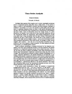
Fig. 2. Architecture of the neural network of the NCSTAR model. The outputs of the network are the coefficients of a linear model. The hidden layer creates multivariate smooth thresholds in the input space. The input variables are called transition variables.

A hyperplane induces a partition of the space into two regions defined by the halfspaces

Fig. 3. initialization procedure in pseudocode.

(7) and (8) associated to the state, activated or not, of the neuron. The norm of is called the slope parameter. In the limit, when the slope parameter approaches infinity, the logistic function becomes an indicator function. With hyperplanes, an -dimensional space will be split into several polyhedral regions. Each region is defined by the nonempty intersection of the halfspaces (7) and (8) of each hyperplane. The main idea of the proposed model is to use (5) to create a smooth multidimensional threshold structure. Suppose that an -dimensional space is spanned by a vector formed by lagged observations of a time series and/or any other exogenous vari, ables, and suppose we have neurons defined by , each of which defines a smooth multivariate threshold. Now consider a time-varying time series model expressed as (9) where parameter vector; ; -dimensional vector of explanatory variables formed and/or any by lagged variables of the time series other exogenous variables. may contain or not common Note that the composition of variables with . The term is a normally distributed white noise with finite, not necessarily constant, variance . The time of (9) is given by the output of evolution of the coefficients a neural network

Fig. 4. Neural-network architecture for learning the error variance with an auxiliary hidden unit. The number of neurons in the auxiliary unit is the same as in the original hidden layer. The error variance is a piecewise constant process with smooth transitions between regimes, controlled by the transition variables.

(10) Fig. 5. Neural-network representation of model (22).



Fig. 6.

Scatter plot of y versus y

and y^ versus y

1405

. The circles are the true values of y and the dots are the estimated y^ .

where and , and , are, respectively, the weights of the synapses between the hidden neurons and the output units of the neural network and the offset parameters of the output units. The neural-network architecture of the NCSTAR model is illustrated in Fig. 2. The elements of , called the transition variables, are the inputs of the neural network. Equations (9) and (10) represent a time-varying model with a multivariate smooth threshold structure defined by hidden neurons. Model (9) can be rewritten as

(11) , and , , . In the case where the variables of the model are just lags of , model (11) is denoted by the acronym ), where and are, respectively, the NCSTAR( and . set of lags that compose

where

IV. RELATIONSHIP BETWEEN THE NCSTAR MODEL AND OTHER NONLINEAR MODELS The idea behind the NCSTAR model is similar to the class of threshold models. The goal is to change the parameters of a linear model according to the value of certain variables. However, in the NCSTAR model the thresholds can be multivariate

and smooth, while in the SETAR model, the thresholds are monovariate and sharp. The SETAR model can only split the input space into subspaces with hyperplanes orthogonal to only one lagged variable of the observed time series, while the NCSTAR model can create hyperplanes in any direction. In the STAR model there is only one threshold, while in the NCSTAR the number of thresholds is not fixed. Finally, the NCSTAR model, as the STAR model, has a formal algorithm to estimate the parameters, while in the SETAR model the algorithm is heuristic.

V. ESTIMATION OF THE PARAMETERS The cost function to be minimized is the sum of the squared errors over all patterns, given by

(12) is the total number of observations and is the eswhere timated value. In this paper, two training algorithms are developed. The first one is the conventional backpropagation adapted to the NCSTAR structure and the second one is a hybrid algorithm that mixes the ordinary least squares (OLS) estimator and nonlinear search, based on the linear property of the output layer.


1406

Fig. 7.


Scatter plot of the coefficients versus y t

0 1.

A. Backpropagation Type Algorithm the th neuron of the hidden layer and th Considering input and the bias of the th neuron of the hidden layer, the parameter-update rule is expressed by

(13)

(14)

Fig. 8. Neural network representation of model (23).

where

is the learning rate parameter.

(15) B. OLS-Nonlinear Search Defining and

, , , (10) can be rewritten as

(16)


(17)


Fig. 9.

Scatter plot of y versus y

Denoting

0 1 and y

versus y

0 1. The circles are the true values of y

and , (9) becomes

, where

(18) Applying the vec1 operator to both sides of (18), and using the vec , we obtain property2 that vec (19) Equation (19) is a linear regression model to which the ordinary least squares estimator can be applied, obtaining

1407

and the dots are the estimated y^ .

The parameters and , can be estimated by the nonlinear search defined in (15) and (16). Summarizing, the estimation algorithm works as follows. and , 1) Choose initial values for the parameters , by the procedure described in Section VI. , and using 2) Estimate the parameters , (20). and , 3) Use (15) and (16) to compute new values for . 4) Repeat Steps 2) and 3) until reaching a (local) minimum of the cost function. This type of algorithm is known in the statistical literature as concentrated least squares [14]. VI. INITIAL CONDITIONS

(20) Sometimes in practice, the matrix does not have an inverse and a pseudoinverse should be calculated by a singular-value decomposition algorithm.

A

2

a B

2

1Let be a (m n) matrix with (m 1) columns . The vec operator transforms into an (mn 1) vector by stacking the columns of . 2 denotes the Kronecker product. Let = (a ) and = (b ) be (m n) and (p q ) matrices, respectively. The (mp nq ) matrix

A

2

A

2

A B =

a . ..

a

is the Kronecker product of

B 111 ..

a . ..

.

B 111

A and B.

2

a

B B

A

2

This section describes a procedure to choose the initial parameters of the hidden layer based on its geometric properties. As shown in Section III, the direction of the weight vector , , determines the orientation of the thresholds and the norm of defines the smoothness of the transition between two half spaces induced by the thresholds. In our procedure the weights of the synapses arriving at the hidden neurons are initialized with the same value, given by a constant times the first ). In that sense, principal component of ( we are assuming that the hyperplanes are parallel and their initial orientation is in the direction perpendicular of the maximum variance of the input variables. The constant is data dependent and in practice we estimate models with different values of .


1408

Fig. 10.


Scatter plot of the coefficients versus y

.

The offset term of each neuron determines the position of the threshold boundary in terms of its distance from the origin. In our procedure they are initialized so as to divide the range of the projections of the data points in direction of the first principal , in equal segments around their mean. Denoting component, by , the pseudocode of the algorithm to inithe mean of is shown in Fig. 3. tialize the vector VII. LOCAL ERROR BARS FOR HETEROSCEDASTIC PROCESSES In this section, we consider the estimation of heterocedastic models where the variance of the error term depends on the same set of input variables as the neural network part of the NCSTAR model. Although this restriction can be easily relaxed, it is specially convenient for us to consider the same set of inputs since they represent the threshold variables of the SETAR models that will be considered in the experiments described in Section VIII. As suggested by Nix and Weigend [22], the variance can be estimated by an auxiliary network attached to the original structure, with which it shares the same inputs. This subnetwork consists of one hidden layer with logistic activation functions and an output layer consisting of one neuron with exponential activation function, representing the local variance. By analogy with the discussion of Section III, this is equivalent to model the variance as a piecewise constant function with smooth transitions between regimes. The final structure for the heterocedastic NCSTAR model is shown in Fig. 4. For the heteroscedastic version of the NCSTAR treated in this section, the

Fig. 11.

Neural-network architecture of model (24).

least squares estimation method described in Section V is no longer optimum. In order to incorporate the variance in the estimation criterion a likelihood function is maximized by a modified backpropagation algorithm. The estimation process is divided into three steps. time-invariant and and train the NCSTAR 1) Consider model with one of the learning algorithms described in Section V, without adding the auxiliary network. 2) Attach the subnetwork and train it to learn the variance. Freeze the parameters estimated in Step 1, and train the output unit to predict the squared errors, using the backpropagation algorithm. 3) Unfreeze all the parameters and train the network to minimize the negative logarithm of the likelihood function



Fig. 12.

1409

Time evolution of the coefficients of the NCSTAR model.

(21) considering Gaussian errors. VIII. EXPERIMENTAL RESULTS In this section we use some computer simulated data to test the performance of the NCSTAR model in identifying SETAR processes. We have simulated three models with 300 observations each one. As our main concern is to test if the NCSTAR model identifies correctly the simulated processes we used all the 300 observations to estimate the parameters. In all the exis a white noise with zero mean and unit amples, the term variance. The experiments were done on a Pentium II computer (400 MHz processor with 256 Mbytes of RAM). The algorithms were programmed in MatLab. A. First Experiment The first simulated time series follows a SETAR(2;1,1) model described by if ; otherwise.

(22)

There are 159 points in the first regime and 141 points in the second regime. It is important to stress that the error variance changes with the regimes.

We fitted an NCSTAR(1;1;1) model with one hidden neuron and with as the input variable of the neural network. Fig. 5 shows the neural-network architecture. and versus Fig. 6 shows the scatter plot of versus with a 95% confidence interval. The training algorithm correctly identifies the threshold position and the change in the variance. Fig. 7 shows the scatter plot of the coefficients of the NCSTAR model versus the transition variable. B. Second Experiment The second simulated time series follows a SETAR(3;1,0,1) model described by

if ; otherwise.

(23)

There are 29 points in the first regime, 249 points in the second regime, and 22 points in the third regime. We fitted an NCSTAR(2;1;1) model with two hidden neurons as the transition variable. Fig. 8 illustrates the and with neural-network architecture. and versus Fig. 9 shows the scatter plot of versus with a 95% confidence interval. The training algorithm correctly captures the dynamics of the data. Fig. 10 shows the scatter plot of the coefficients of the NCSTAR model versus the transition variable.


1410

Fig. 13.


Scatter plot of the coefficients versus y

0y

.

TABLE I IN-SAMPLE RESULTS

C. Third Experiment The third simulated time series follows a SETAR(2;2,2) model with multivariate thresholds described by if otherwise.

;

(24) In this example the error variance does not change with the regimes. There are 161 points in the first regime and 139 points in the second regime. We fitted an NCSTAR(1;1,2;1,2) model with one hidden and as the transition variables. neuron and with Fig. 11 shows the neural-network architecture. Figs. 12 and 13 show the time evolution of the coefficients and the scatter plot of the coefficients of the NCSTAR model . The NCSTAR model correctly captures the versus dynamics of the data. IX. REAL APPLICATION Now the task is to forecast a real time series. We used the annual sunspot number index from 1700 to 1998 (299 obser-

vations). The observations for the period 1700–1979 (280 observations) were used to estimate the models and the remaining (19 observations) were used to forecast evaluation. The sunspot number index is a measure of the area of solar surface covered by spots. The sunspot number index is also known as the Wolf number in reference of the Swiss astronomer J. R. Wolf who first introduced this index in 1848. The sunspot number is a benchmark time series in nonlinear modeling. Several models have been fitted along the years [6], [8], [10], [11], [23], [24], [27]–[29], [33]. In this paper, we adopted the same transformation as in [28], , where is the sunspot number. We compare the performance of the NCSTAR model with the SETAR(2;10,2) model proposed by Tong [28], the linear autoregressive model of order 9, AR(9), and an artificial neural network (ANN) model with five hidden neurons and the first nine lags as input variables and estimated with Bayesian regularization [16], [17]. We estimated a NCSTAR model with three hidden neurons, lags 1 and 2 as transition variables, and the first nine lags of composing the vector . The choice of the elements of was based on previous results in the literature. The number of hidden units and the choice of the transition variables were based on the estimation of several different models. We chose the one with the best out-of-sample performance. Table I shows the standard deviation of the in-sample residuals. As we can see, the NCSTAR has the lowest residual standard deviation.



TABLE II ONE-STEP AHEAD FORECASTS, THEIR ROOT MEAN SQUARE ERRORS, AND MEAN ABSOLUTE ERRORS FOR THE PERIOD 1980 TO 1998

We continue considering the out-of-sample performance of the estimated model. Table II shows, for each model, their one-step ahead forecasts, the respective forecast error, their root mean squared errors (RMSEs), and mean absolute errors (MAEs) for annual number of sunspots for the period 1980 to 1998. Both the RMSE and the MAE of the NCSTAR model are lower than the ones of the concurrent specifications. In that sense, the NCSTAR model outperforms the other formulations. X. CONCLUSIONS This article presents a new alternative to nonlinear modeling, where the coefficients of a linear model are the outputs of a neural network with only one hidden layer. The proposed model, called NCSTAR, is based on the geometrical features of a layer of hidden neurons. The paper shows that the NCSTAR model generalizes the TAR model, by allowing multivariate thresholds and a smooth switching between regimes and has a good performance both with simulated and real data. Although not discussed here, the ideas presented in [2] can useful to select the variables of the model and the number of hidden neurons. Considering the problem of local minima, the use of algorithms like the Broyden–Fletcher–Goldfarb–Shanno (BFGS) algorithm [3, p. 134–140] or the Levenberg–Marquardt [13], [19] in combination with the OLS algorithm described in Section V-B can improve the performance of the training process. ACKNOWLEDGMENT The authors would like to thank C. E. Pedreira, C. Fernandes, G. Veiga, an associate editor, and two anonymous referees for useful suggestions.

1411

FOR THE

ANNUAL NUMBER OF SUNSPOTS

REFERENCES [1] H. Akaike, “Information theory and an extension of the maximum likelihood principle,” in Second International Symposium on Information Theory, B. N. Petrov and F. Czáki, Eds. Budapest, Hungary: Akademiai Kiadó, 1973, pp. 267–281. [2] U. Anders and O. Korn, “Model, selection in neural networks,” Neural Networks, vol. 12, pp. 309–323, 1999. [3] D. P. Bertsekas, Nonlinear Programming. Belmont, CA: Athena, 1995. [4] C. M. Bishop, Neural Networks for Pattern Recognition. Oxford, U.K.: Oxford Univ. Press, 1995. [5] G. E. P. Box, G. M. Jenkins, and G. C. Reinsel, Time Series Analysis, Forecasting and Control, 3rd ed. Englewood Cliffs, NJ: Prentice-Hall, 1994. [6] P. A. Cartwright, “Forecasting time series: A comparative analysis of alternative classes of time series models,” J. Time Series Anal., vol. 6, pp. 203–211, 1985. [7] K. S. Chan and H. Tong, “On estimating thresholds in autoregressive models,” J. Time Series Anal., vol. 7, pp. 179–190, 1986. [8] C. W. J. Granger and A. P. Andersen, An Introduction to Bilinear Time Series Models. Gottingen: Vandenhoek and Ruprecht, 1978. [9] C. W. J. Granger and T. Teräsvirta, Modeling Nonlinear Economic Relationships. Oxford, U.K.: Oxford Univ. Press, 1993. [10] V. Haggan, S. M. Heravi, and M. B. Priestley, “A study of the application of the state-dependent autoregressive tune series model,” Biometrika, vol. 68, pp. 189–196, 1984. [11] V. Haggan and T. Ozaki, “Modeling nonlinear random vibrations using an amplitude-dependent autoregressive time series model,” Biometrika, vol. 68, pp. 189–196, 1981. [12] H. Haykin, Neural Networks: A Comprehensive Foundation, 2nd ed. Englewood Cliffs, NJ: Prentice-Hall, 1999. [13] K. Levenberg, “A method for the solution of certain problems in least squares,” Quart. Appl. Math., vol. 2, pp. 164–168, 1944. [14] S. Leybourne, P. Newbold, and D. Vougas, “Unit roots and smooth transitions,” J. Time Series Anal., vol. 19, pp. 83–97, 1998. [15] S. Lundbergh, T. Teräsvirta, and D. van Dijk, “Time-varying smooth transition autoregressive models,” in Working Paper Series in Economics and Finance 376. Stockholm, Sweden: Stockholm School of Economics, 2000. [16] D. J. C. MacKay, “Bayesian interpolation,” Neural Comput., vol. 4, pp. 415–447, 1992. [17] , “A practical Bayesian framework for backpropagation networks,” Neural Comput., vol. 4, pp. 448–472, 1992.


1412

[18] Y. Makamori and M. Ryoke, “Identification of fuzzy prediction models through hyperellipsoidal clustering,” IEEE Trans. Syst., Man, Cybern., vol. 24, pp. 1153–1173, 1994. [19] D. Marquardt, “An algorithm for least-squares estimation of nonlinear parameters,” SIAM J. Appl. Math., vol. 11, pp. 431–441, 1963. [20] M. C. Medeiros, “Hibrid linear-neural model for time series analysis and forecasting,” Master’s thesis (in Portuguese), Catholic Univ., Rio de Janeiro, Brazil, 1998. [21] M. T. N. Mellem, “Hybrid autoregressive-neural models for titre series,” Master’s thesis (in Portuguese), Catholic University, Rio de Janeiro, Brazil, 1997. [22] D. A. Nix and A.S. Weigend, “Learning local error bars for nonlinear regression,” in Advances in Neural Information Processing Systems 7 (NIPS*94), D. S. Touretzky, G. Tesauro, and T. K. Leen, Eds. Cambridge, MA,: MIT Press, 1995. [23] J. Pemberton, “Contributions to the theory of nonlinear titre series models,” Ph.D. dissertation, Univ. Manchester, Manchester, U.K., 1985. [24] T. Subba Rao and M. M. Gabr, “An introduction to bispectral analysis and bilinear time series models,” in Lecture Notes in Statistics. New York: Springer-Verlag, 1984, vol. 24. [25] T. Teräsvirta, “Specification, estimation, and evaluation of smooth transition autoregressive models,” J. Amer. Statist. Assoc., vol. 89, no. 425, pp. 208–218, 1994. [26] H. Tong, “On a threshold model,” in Pattern Recognition and Signal Processing, C. H. Chen, Ed. Amsterdam, The Netherlands: Sijthoff and Noordhoff, 1978. , “Threshold models in nonlinear time series analysis,” in Lecture [27] Notes in Statistics. New York: Springer-Verlag, 1983, vol. 21. [28] , “Non-linear time series: A dynarnical systetrls approach,” in Oxford Statistical Science Series. Oxford, U.K.: Oxford Univ. Press, 1990, vol. 6. [29] H. Tong and K. S. Lim, “Threshold autoregression, limit cycles and cyclical data (with discussion),” J. Roy. Statisti. Soc., ser. B 42, pp. 245–292, 1980. [30] R. S. Tsay, “Testing and modeling threshold autoregressive processes,” J. Amer. Statist. Assoc., vol. 84, pp. 431–452, 1989. [31] D. van Dijk and P. H. Franses, “Modeling multiple regimes in the business cycle,” Macroecon. Dyn., vol. 3, no. 3, pp. 311–340, 1999.


[32] A. Veiga and M. C. Medeiros, “A hybrid linear-neural model for time series forecasting,” in Proc. NEURAP 98, Marseilles, France, 1998, pp. 377–384. [33] A. S. Weigend, B. A. Huberman, and D. E. Rumelhart, “Predicting sunspots and exchange rates with connectionist networks,” in Nonlinear Modeling and Forecasting, M. Casdagli and S. Eubank, Eds. MA: Addison-Wesley, 1992. [34] G. Zhang, B. E. Patuwo, and M. Y. Hu, “Forecasting with artificial neural networks: The state of the art,” Int. J. Forecasting, vol. 14, pp. 35–62, 1998.

Marcelo Medeiros was born in Rio de Janeiro, RJ, Brazil, in 1974. He received the B.S. degree in electrical engineering (systems), and the M.S. and the Ph.D. degrees from the Catholic University of Rio de Janeiro (PUC-Rio) in 1996, 1998, and 2000. His main research interest is nonlinear time series modeling.

Álvaro Veiga was born in Florianbpólis, SC, Brazil, in 1955. He received the B.S. degree in electrical engineering (systems) from the Catholic University of Rio de Janeiro (PUC-Rio) in 1978, the M.S. degree from COPPE-UFRJ, Rio de Janeiro, in 1982, and the Ph.D. degree from the École Nationale Supérieure des Télécommunications, Paris, France, in 1989. Since 1990, he has been at the Catholic University of Rio de Janeiro as an Assistant Researcher/Professor. His main research interests include nonlinear modeling and data analysis with application to finances, energy, and learning achievement analysis.
