A Hybrid Model of Evolutionary Algorithms and Branch-and-Bound for ...

A Hybrid Model of Evolutionary Algorithms and Branch-and-Bound for Combinatorial Optimization Problems Jos´e E. Gallardo, Carlos Cotta, Antonio J. Fern´andez Dept. Lenguajes y Ciencias de la Computaci´on, Universidad de M´alaga ETSI Inform´atica, Campus de Teatinos 29071 - M´alaga - Spain {pepeg,ccottap,afdez}@lcc.uma.es Abstract- Branch-and-Bound and evolutionary algorithms represent two very different approaches for tackling combinatorial optimization problems. These approaches are not incompatible though. In this paper, we consider a hybrid model that combines these two techniques. To be precise, it is based on the interleaved execution of both approaches, and has a heuristic nature. The multidimensional 0-1 knapsack problem has been chosen as benchmark. As it will be shown, the hybrid algorithm can produce better results at the same computational cost, specially for larger problem instances.

1 Introduction Branch-and-bound techniques (BnB) [LW66] constitute a well-known approach for solving combinatorial optimization problems to optimality. Essentially, BnB techniques produce upper and lower bounds that eventually converge to the optimal solution. To this end, an implicit enumeration scheme is used: the algorithm starts with a problem (or node) that represents the whole search space; subsequently, it proceeds iteratively by picking a node, and dividing it into mutually excluding subproblems that represent a partition of the original search space. Upper and lower bounds are computed for these subproblems; then, they are successively divided until they can be trivially solved, or until their upper bound is lower than the best known solution (maximization assumed). Thus, the search performed by the algorithm can be represented as a tree. This tree can be traversed in several ways. The most efficient (in terms of the number of iterations) is best-first, i.e., expanding firstly the most promising –according to the upper bound– nodes. However, the memory requirements can make this strategy unrealistic for large problem instances. The alternative is using a depthfirst traversal. This strategy does not require large amounts of memory, but can expand much more nodes than best-first. On the other hand, evolutionary algorithms (EAs) [B¨ac96, BFM97] have a completely different philosophy: tentative solutions are iteratively generated, aiming at producing better and better solutions. Their performance is probably, yet not provably, good: near-optimal solutions can be typically found at an acceptable computational cost in many combinatorial optimization problems. It must be noted that –despite the underlying algorithmic template of EAs being fairly the same in these different problems– the need for exploiting problem-knowledge has been repeatedly shown in theory and in practice [Cul98, Dav91, WM97]. Problem-knowledge can be incorporated to an EA in many ways. A popular option is the hybridization of the

algorithm with some problem-specific technique. In this sense, we here present a model for hybridizing EAs with BnB techniques. The goal is combining synergistically these two different solving approaches, exploiting the capability of BnB for identifying provably good regions of the search space, and the power of EAs for exploring these. Before detailing how this is precisely achieved, let us firstly describe the underlying search techniques that will be combined. This will be done in the context of the multidimensional 0-1 knapsack problem (MKP).

2 Exact and Evolutionary Approaches to the MKP The MKP is a generalization of the classical 0-1 knapsack problem, so it is worth describing the latter in the first place. Subsequently, the algorithmic approaches considered for tackling the MKP will be shown. 2.1 The Multidimensional 0-1 Knapsack Problem An instance of the classical 0-1 knapsack problem is defined by a knapsack of capacity b, and a set of n objects O = {o1 , · · · , on }. Each of these objects oj has a value pj and a weight rj . The problem amounts to selecting a subset S ⊆ O of objects, such that their combined weight does not exceed the knapsack capacity, and their value is maximal. The MKP generalizes the previous definition by considering m different knapsacks, each of them with a possibly different capacity bi . The subset of objects selected must fit simultaneously within all m knapsacks. Furthermore, objects have a different weight rij within each knapsack1 . This way, the problem can be formalized as follows: maximize Pn j=1

subject to Pn

pj xj ,

j=1 rij xj ≤ bi , xj ∈ {0, 1},

i = 1, . . . , m, j = 1, . . . , n.

and pj > 0, rij ≥ 0, bi ≥ 0 Thus, vector ~x describes the objects selected in the solution. The problem is strongly-NP [GJ79], and does not 1 An alternative interpretation of the problem is considering these knapsacks as different resources, being bi the available amount of resource i, and rij the consumption of resource i by object j.

admit a fully polynomial time approximation scheme (FPTAS) [KS81]. It can be regarded as a general statement of binary integer programming with non-negative coefficients. Many real-world problems can be formulated as the MKP, e.g., capital budgeting, project selection, (see [SM89] for instance). 2.2 A BnB Approach to the MKP The BnB algorithm considered carries out a standard exploration of the search tree for this kind of problems (see [BM80]). More precisely, the linear relaxation of each node is solved (i.e., the corresponding subproblem is solved assuming variables can take fractional values in the interval [0,1]) using linear-programming (LP) techniques. If all variables take integral values, the subproblem is solved. This is not generally the case though, and some variables are non-integer in the LP-relaxed solution; in the latter situation, the variable whose value is closest to 0.5 is selected, and two subproblems are generated, fixing this variable to 0 or to 1 respectively. The LP-relaxed value of the node is used as its upper-bound, so that nodes whose value is below the best-known solution can be pruned from the search tree. The tree can be traversed in different ways as mentioned in Section 1. If a depth-first strategy is used, the memory required grows linearly with the depth of the tree; hence large problems can be considered. However, the timeconsumption can be excessive. On the other hand, a bestfirst strategy minimizes the number of nodes explored, but the size of the search tree (that is, the number of nodes kept for latter expansion) will grow exponentially in general. A third option is using a breadth-first (or level-order) traversal. In principle, this option would have the drawbacks of the previous two strategies, unless a heuristic choice is made: keep at each level just the best k nodes. This implies sacrificing exactness, but provides a very effective heuristic search approach. The name beam search has been coined to denote this strategy. We have precisely used this approach in our hybrid model. 2.3 An EA for the MKP The MKP has been tackled via EAs in many works, e.g., [KBH94, Rai98, CB98, CT98, Got00, RG04]. Among these, the EA developed by Chu and Beasley [CB98] remains as one of the cutting-edge approaches for solving the MKP. This EA uses the natural codification of solutions, namely binary n-dimensional strings ~x, representing the incidence vector of a subset S of objects on the universal set O (i.e., (xj = 1) ⇔ oj ∈ S). Of course, infeasible solutions could be encoded in this way, so a repairing algorithm is used. To do so, an initial pre-processing of the problem instance is performed offline. The goal is obtaining a heuristic precedence order among variables: they are ordered for decreasing pseudoutility values (see [CB98] for details). Variables near the front of this ordered list are more likely to be latter included in feasible solutions (and analogously, variables near the end of the list are more likely to be excluded from feasible

initialize Ri =

Pn

j=1 rij xj , ∀i

∈ {1, · · · , n};

/* DROP phase */

for j = n down to 1 do if (xj = 1) and (∃i ∈ {1, · · · , m} : Ri > bi ) then set xj ← 0; set Ri ← Ri − rij , ∀i ∈ {1, · · · , m} end if end for /* ADD phase */

for j = 1 up to n do if (xj = 0) and (∀i ∈ {1, · · · , m} : Ri + rij ≤ bi ) then set xj ← 1; set Ri ← Ri + rij , ∀i ∈ {1, · · · , m} end if end for Figure 1: Repairing/improving algorithm used in the EA. solutions). Once the heuristic ordering is produced, a two-phase repairing algorithm is applied to each solution (see Figure 1). In the first phase, variables are examined in increasing order of pseudo-utility, and changed to 0 while the solution is infeasible. In the second phase, variables are examined in reverse order and changed to 1 as long as feasibility is kept. Therefore, the goal of the first phase is attaining feasibility, while the goal of the second phase is improving the quality of solutions. Since this EA just explores the feasible portion of the search space, Pn the fitness function can be readily defined as f (~x) = j=1 pj xj .

3 Hybrid Models In this section we present a hybrid model that integrates an EA with a BnB algorithm. Our aim is to combine the advantages of both approaches and, at the same time, reduce their drawbacks working alone. Firstly, in the following subsection, we briefly discuss some related works existing in the literature regarding the hybridization of EA techniques and BnB algorithms. 3.1 Related Work Cotta et al. [CANT95] used a problem-specific BnB approach for the traveling salesman problem based on 1-trees and the Lagrangean relaxation [VJ82], and made use of an EA to provide bounds in order to guide the BnB search. More specifically, two different approaches for the integration were analyzed. In the first model, the genetic algorithm played the role of master and the BnB was incorporated as a slave. The primary idea was to build a hybrid recombination operator based in the BnB philosophy. More precisely, the BnB was used in order to build the best possible tour within the (Hamiltonian) subgraph defined by the union

of edges in the parents. This recombination procedure was costly, but provided better results than blind edge recombination. The second model proposed consisted of executing in parallel the BnB algorithm with a certain number of EAs which generated a number of different high-quality solutions. The diversity provided by the independent EAs contributed to make that edges suitable to be part of the optimal solution were likely included in some individuals, and nonsuitable edges were unlikely taken into account. Despite these approaches showed encouraging results, the work in [CANT95] described only preliminary results. Another relevant research was developed by Nagar et al. [NHH96], combining a BnB tree search and an EA which was used to provide bounds for solving flowshop scheduling problems. Later, a hybrid algorithm, combining genetic algorithms and integer programming BnB approaches to solve MAX-SAT problems was described by French et al. [FRW01]. This hybrid algorithm gathered information during the run of a LP-based BnB algorithm, and used it to build the population of an EA population. The EA was eventually activated, and the best solution found was used to inject new nodes in the BnB search tree. The hybrid algorithm was run until the search tree was exhausted, and hence it is an exact approach. However, in some cases it expands more nodes than the BnB algorithm alone. More recently, Cotta and Troya [CT03] presented a framework for the hybridization along the lines initially sketched in [CANT95], i.e., based on using the BnB algorithm as a recombination operator embedded in the EA. This hybrid operator is used for recombination: it intelligently explores the possible children of solutions being recombined, providing the best possible outcome. The resulting hybrid algorithm provided better results than pure EAs in several problems where a full BnB exploration was unpractical on its own. In [GCF05], we presented another hybrid algorithm that keeps some similarities with the new one that we describe in Section 3.2. One of the differences with the algorithm presented in this paper is that in [GCF05] we used an EA that enabled the appearance of duplicated individuals in the population. Also, the BnB algorithm in [GCF05] was less sophisticated and did not make use of the linear relaxation of the problem to obtain upper bounds (as we do now). Moreover, the search tree was traversed by expanding firstly the more promising nodes, and node bounds were not employed to guide the search of the EA. Last, but not least, the former approach was intended to be a complete anytime algorithm. However, it may be worth trading completeness for improved accuracy, as it will be shown henceforth. 3.2 Our Hybrid Algorithm One way to do the integration of evolutionary techniques and BnB models is via a direct collaboration that consists of letting both techniques work alone in parallel (i.e., let both processes perform independently), that is, at the same level. By doing so, both processes will share the solution (see Fig. 2) so that we can obtain the following benefits: • The BnB can use the current solution to purge the

Lower bounds

EA

BnB Algorithm

Promising regions

Figure 2: A model for algorithmic collaboration. problem queue, deleting those problems whose upper bound is smaller than the one obtained by the EA. • The BnB can inject information about more promising regions of the search space into the EA population in order to guide the EA search. The hybrid algorithm starts by running the EA in order to obtain a first approximation to the solution. In this initial phase, the population is randomly initialized and the EA executed until the solution is not improved for a certain number of iterations. Afterwards, a version of the BnB algorithm that expands the search tree in a breadth-first way is executed (i.e., every node in a level is explored before moving to the next). To avoid an excessive memory consumption (and to save the computational time of computing the LP-relaxed solution for some nodes), in each level of the search tree we only consider the k more promising nodes. The EA is then executed during the transition of levels in the search tree (i.e., when the search tree grows in depth). For executing the EA, the population initialization takes into account the set of k nodes in the current level of the search tree of the BnB algorithm. Note that these nodes actually represent schemata, i.e., they are partial solutions in which some bits are fixed but another ones are indeterminate. These schemata are converted in full solutions as follows: for each schemata s in the BnB node-list do for i = 1 up to n do if si =* then set xi ← Rand{0,1}; else set xi ← si end if end for repair x inject x in the population end for The resulting solutions are incorporated into the EA population. The intended goal of this process is to lead the EA search to these regions of the search space (recall that the

Figure 3: Sketch of the hybrid algorithm. nodes in the queue represent subsets of the search space considered promising by the BnB; hence, the EA is used for finding probably good solutions in this region). The EA evaluation function in this stage is modified to be n X z(~x) f (~x) = pj xj + , (1) 2 j=1 where z(~x) is the upper bound of the best open node (i.e., currently considered in the BnB algorithm) that is compatible2 with ~x, or 0 in case no node is compatible. Doing so, those EA individuals that belong to the more promising regions will obtain better aptitude value, and as consequence, it is expected that the exploration will probably be focused on those regions. The 1/2 factor in this equation is a mere scale term, adjusted in preliminary experiments. Upon stabilization of the EA, control is returned to the BnB algorithm. The lower bound for the optimal solution obtained by the EA is then compared to the current incumbent in the BnB, updating the latter if necessary. This may lead to new pruned branches in the BnB search tree. This is repeated until the search tree is exhausted, or a time limit is reached. The whole process is illustrated in Figure 3.

4 Experimental Results We have tested our algorithms with problems available at the OR-library [Bea90] maintained by Beasley. We took two instances per problem set. Each problem instance is characterized by a number m of constraints (or knapsacks), a number n of items and a tightness ratio, 0 ≤ α ≤ 1. The closer to 0 the tightness ratio the more constrained the instance. To be precise, the capacity of the i-th knapsack is 2 A node is compatible with respect to a solution if all bits specified in the node coincide with those in the solution.

bi = α

n X

rij .

(2)

j=1

We solved these problems on a Pentium IV PC (1700MHz and 256MB of main memory) using the EA, three different BnB algorithms –using depth-first, best-first, and beam search (k = 100)–, and the hybrid algorithm (all of them coded in C). A single execution for each instance was performed for the three BnB methods (since these are exact methods) whereas ten independent runs per instance were carried out for the EA and hybrid algorithms. The algorithms were run for 600 seconds in all cases. For the EA and the hybrid algorithm, the size of the population was fixed at 100 individuals that were initialized with random feasible solutions. With the aim of maintaining some diversity in the population, duplicated individuals were not allowed in the population. The crossover probability was set to 0.9, binary tournament selection was used, and standard uniform crossover operator was chosen. Execution results for BnB algorithms are shown in Tables 1-3. The first three columns indicate the tightness ratio (α), and the sizes (m and n) for a particular instance. The next column reports results for the best solution found as well as the time (in seconds) consumed to find it. Specifically for the EA and hybrid algorithms, in Tables 4 and 5 we also show the mean of the values obtained and standard deviations, and the average time to obtain the best solution. For clarity, the best results obtained globally (excluding ties) are written in bold face. Since the EA and the hybrid algorithm are stochastic techniques, we have considered the mean value for comparisons between them. When comparing to the deterministic BnB algorithms, we have considered the best solution though. As it can be seen, the hybrid algorithm provides better results for the largest problem instances ({10, 30} × 500 and 30 × 250), regardless of the tightness ratio. For the smallest problem instances, the pure EA performs better. This

5

5

1.16

x 10

3.0715

x 10

hybrid algorithm

3.071

1.159 EA beam search

3.0705 best solution found

best solution found

1.158

1.157

3.0695

1.155

3.069

0

100

200

300 time (s)

400

500

600

beam search

3.07

1.156

1.154

hybrid EA

3.0685

0

100

200

300 time (s)

400

500

600

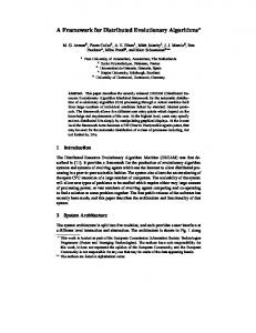
Figure 4: Evolution of the best solution in the evolutionary algorithm (EA), beam search, and the hybrid algorithm during 600 seconds of execution. (Left) problem instance with α = .25, m = 30, n = 500. (Right) problem instance with α = .75, m = 10, n = 500. In both cases, curves are averaged for ten runs for the EA and the hybrid algorithm.

α

m

0.25

10

30

0.75

10

30

n 100 250 500 100 250 500 100 250 500 100 250 500

solution 23064 59187 117733 21946 56702 115857 60633 149685 307072 60603 149595 300473

t 126.04 481.25 334.37 3.82 21.10 268.09 0.64 19.12 10.13 16.54 216.10 465.43

Table 1: Results of the BnB algorithm with depth-first exploration.

α

m

0.25

10

30

0.75

10

30

n 100 250 500 100 250 500 100 250 500 100 250 500

solution 23064 59187 117779 21946 56824 115857 60633 149704 307072 60603 149595 300473

t 16.61 35.60 429.34 1.37 468.12 153.64 0.21 293.28 594.92 2.64 23.75 134.43

Table 2: Results of the BnB algorithm with best-first exploration.

α

m

0.25

10

30

0.75

10

30

n 100 250 500 100 250 500 100 250 500 100 250 500

solution 23057 59133 117772 21946 56824 115795 60633 149641 307013 60603 149595 300512

t 2.37 8.25 67.23 1.09 14.35 554.37 0.29 0.54 31.67 5.03 45.43 198.73

Table 3: Results of the BnB algorithm with beam-search.

α

m

0.25

10

30

0.75

10

30

n 100 250 500 100 250 500 100 250 500 100 250 500

best 23064 59187 117772 21946 56824 115894 60633 149704 307050 60603 149601 300531

mean ± σ 23064 ± 0 59180.3 ± 7.4 117743.6 ± 21.8 21946 ± 0 56767.0 ± 53.9 115847.7 ± 31.4 60633 ± 0 149704 ± 0 307032.3 ± 20.6 60603 ± 0 149594.4 ± 4.8 300484.9 ± 23.1

t 17.5 342.4 277.6 2.1 250.2 303.9 1.1 91.7 175.4 68.9 197.5 199.8

Table 4: Results of Chu and Beasley’s EA.

α

m

0.25

10

30

0.75

10

30

n 100 250 500 100 250 500 100 250 500 100 250 500

best 23064 59166 117772 21946 56824 116014 60633 149704 307050 60603 149601 300531

mean ± σ 23057.7 ± 2.1 59161.7 ± 7.5 117764.3 ± 15.7 21946 ± 0 56824 ± 0 115911.8 ± 52.4 60633 ± 0 149696.3 ± 12.8 307038.9 ± 16 60603 ± 0 149595.4 ± 1.9 300491.5 ± 20.7

t 2.5 76.8 165.1 1.1 174.6 253.5 0.6 26.4 187.9 48.6 433.7 266.9

Table 5: Results of the hybrid algorithm. Entries in italics indicate that the hybrid algorithm provided the best results ex aequo with another algorithm(s). may be due to the lower difficulty of the latter instances; the search overhead of switching from the EA to the BnB may not be worth in this case. The hybrid algorithm just starts being advantageous in larger instances, where the EA faces a more difficult optimization scenario. With respect to the BnB algorithms, notice that the hybrid algorithm always provides better solutions than beam search, and similar or better solutions than that of the other BnB algorithms. Of course, the results of these latter algorithms must be taken as just indicative, since no hybridization with depth-first BnB or best-first BnB has been attempted here. Figure 4 shows the evolution of the best value found by the different algorithms for two specific problem instances. Note that the hybrid algorithm always provides here better results than the original ones, specially in the case of the more constrained instance (α = .25).

5 Conclusions and Future Work We have presented a hybridization of an EA with a BnB algorithm. The EA provides lower bounds that the BnB algorithm can use to purge the problem queue, whereas the BnB guides the EA to look into promising regions of the search space. The resulting hybrid algorithm has been tested on large instances of the MKP problem with encouraging results: the hybrid EA produces better average results than the constituent algorithms on specific instances. This indicates the synergy of this combination, thus supporting the idea that this is a profitable approach for tackling difficult combinatorial problems. In this sense, further work will be directed to confirm these findings on different combinatorial problems, as well as to study alternative models for the hybridization of the BnB with EAs. Another very interesting line for future developments refers to the parallelization of the hybrid algorithm. Several possibilities can be considered here. On one hand, any of the constituent algorithms can be internally parallelized; for instance, the EA can use an island-based model, or we can distribute the evaluation of nodes in the current level among a number of computers. This can lead to improved results

due to the numerical speed-up in the BnB part, and the algorithmic speed-up in the EA component [CP00]. On the other hand, a fully asynchronous functioning of both components (EA and BnB) with occasional communication is a very appealing option for dealing with large-scale optimization tasks.

Acknowledgements This work was partially supported by Spanish MCyT under contracts TIC2002-04498-C05-02 and TIN2004-7943-C0401. Thanks are due to one of the anonymous reviewers for useful comments that have enhanced the readability of the article.

Bibliography [B¨ac96]

T. B¨ack. Evolutionary Algorithms in Theory and Practice. Oxford University Press, New York NY, 1996.

[Bea90]

J.E. Beasley. Or-library: distributing test problems by electronic mail. Journal of the Operational Research Society, 41(11):1069–1072, 1990.

[BFM97]

T. B¨ack, D.B. Fogel, and Z. Michalewicz. Handbook of Evolutionary Computation. Oxford University Press, New York NY, 1997.

[BM80]

E. Balas and H. Martin. Pivot and Complement - a heuristic for 0-1 programming. Management Science, 26(1):86–96, 1980.

[CANT95] C. Cotta, J.F. Aldana, A.J. Nebro, and J.M. Troya. Hybridizing genetic algorithms with branch and bound techniques for the resolution of the TSP. In D.W. Pearson, N.C. Steele, and R.F. Albrecht, editors, Artificial Neural Nets and Genetic Algorithms 2, pages 277–280, Wien New York, 1995. Springer-verlag. [CB98]

P.C. Chu and J.E. Beasley. A genetic algorithm for the multidimensional knapsack problem. Journal of Heuristics, 4:63–86, 1998.

[CP00]

E. Cant´u-Paz. Efficient and Accurate Parallel Genetic Algorithms, volume 1 of Genetic Algorithms and Evolutionary Computation. Kluwer Academic Publishers (now Springer-Verlag), 2000.

[CT98]

C. Cotta and J.M. Troya. A hybrid genetic algorithm for the 0-1 multiple knapsack problem. In G.D. Smith, N.C. Steele, and R.F. Albrecht, editors, Artificial Neural Nets and Genetic Algorithms 3, pages 251–255, Wien New York, 1998. Springer-Verlag.

[CT03]

C. Cotta and J.M. Troya. Embedding branch and bound within evolutionary algorithms. Applied Intelligence, 18(2):137–153, 2003.

[Cul98]

J. Culberson. On the futility of blind search: An algorithmic view of “no free lunch”. Evolutionary Computation, 6(2):109–128, 1998.

[Dav91]

L. Davis. Handbook of Genetic Algorithms. Van Nostrand Reinhold, New York NY, 1991.

[FRW01]

A.P. French, A.C. Robinson, and J.M. Wilson. Using a hybrid genetic-algorithm/branch and bound approach to solve feasibility and optimization integer programming problems. Journal of Heuristics, 7(6):551–564, 2001.

[GCF05]

J.E. Gallardo, C. Cotta, and A.J. Fern´andez. Solving the multidimensional knapsack problem using an evolutionary algorithm hybridized with branch and bound. In Artificial Intelligence and Knowledge Engineering Applications: A Bioinspired Approach, number 3562 in Lecture Notes in Computer Science, pages 21– 30, Berlin Heidelberg, 2005. Springer-Verlag. In press.

[GJ79]

M.R. Garey and D.S Johnson. Computers and Intractability: A Guide to the Theory of NPCompleteness. Freeman and Co., San Francisco CA, 1979.

[Got00]

J. Gottlieb. Permutation-based evolutionary algorithms for multidimensional knapsack problems. In J. Carroll, E. Damiani, H. Haddad, and D. Oppenheim, editors, ACM Symposium on Applied Computing 2000, pages 408–414. ACM Press, 2000.

[KBH94]

S. Khuri, T. B¨ack, and J. Heitk¨otter. The zero/one multiple knapsack problem and genetic algorithms. In E. Deaton, D. Oppenheim, J. Urban, and H. Berghel, editors, Proceedings of the 1994 ACM Symposium on Applied Computation, pages 188–193. ACM Press, 1994.

[KS81]

B. Korte and R. Schrader. On the existence of fast approximation schemes. In O.L. Mangasarian, R.R. Meyer, and S. Robinson, editors, Nonlinear Programming 4, pages 415–437. Academic Press, 1981.

[LW66]

E.L. Lawler and D.E. Wood. Branch and bounds methods: A survey. Operations Research, 4(4):669–719, 1966.

[NHH96]

A. Nagar, S.S. Heragu, and J. Haddock. A combined branch and bound and genetic algorithm based for a flowshop scheduling algorithm. Annals of Operation Research, 63:397–414, 1996.

[Rai98]

G.R. Raidl. An improved genetic algorithm for the multiconstraint knapsack problem. In Proceedings of the 5th IEEE International Conference on Evolutionary Computation, pages 207– 211, 1998.

[RG04]

G.R. Raidl and J. Gottlieb. Empirical analysis of locality, heritability and heuristic bias in evolutionary algorithms: A case study for the multidimensional knapsack problem. Technical Report TR 186–1–04–05, Institute of Computer Graphics and Algorithms, Vienna University of Technology, 2004.

[SM89]

H. Salkin and K. Mathur. Foundations of Integer Programming. North Holland, 1989.

[VJ82]

A. Volgenant and R. Jonker. A branch and bound algorithm for the symmetric traveling salesman problem based on the 1-tree relaxation. European Journal of Operational Research, 9:83–88, 1982.

[WM97]

D.H. Wolpert and W.G. Macready. No free lunch theorems for optimization. IEEE Transactions on Evolutionary Computation, 1(1):67– 82, 1997.