2009 International Symposium on Nonlinear Theory and its Applications NOLTA'09, Sapporo, Japan, October 18-21, 2009
A Hybrid Modeling and Dynamics of Virtual Microgrid under Balancing Restriction Yu Takatsuji† and Takashi Hikihara‡ †‡ Department of Electrical Engineering, Kyoto University Katsura, Nishikyo, Kyoto, 615-8510 JAPAN Email: †
[email protected], ‡
[email protected] Abstract—Microgrid is one of the structures for connecting dispersed power sources with local loads in power network. The islanding state is the exceeded idea for power supply, then the virtual grouping networking is considered to introduce microgrids into conventional accomplished power networks. In order to keep the safety operation of micro-generators in microgrid, switching strategies for generators have been applied but not discussed from the standpoint of dynamics. In this paper, the dynamics of the virtual microgrid is modeled by a hybrid automaton under control for keeping the balancing restriction of power flow. It is shown that the hybrid control is effective to keep the system in safe at realistic level. 1. Introduction Recently, new energy supply systems, consisting of dispersed generations cooperated with power networks, are actively discussed. This might solve issues related to reduction of CO2 emissions and safety energy supply. However, there still exist various problems in the interconnection of numbers of dispersed generations to conventional power systems. For example, natural energy power sources, such as photovoltaic cells and wind turbines, disturb the balance of power supply and demand in the networks because of their power fluctuation. Furthermore, reverse power flows to the upper systems are sensitive for the setting of protective relay and short-circuit capacity. The concept of microgrid seems one of the solutions for them [1]. A microgrid consists of dispersed generators, energy storage systems, loads and a central control center. The center can control power sources and maintain the balance of power supply and demand properly with sensing every flows. Here we introduce a virtual microgrid with conventional power network. Virtual microgrid requests the power behavior between dispersed power sources and supposed loads in a power network. It is important to prevent the continuous unbalance of the power flow in the network for keeping the system behavior in a stable region at a time interval. However, the balancing method cannot overwhelm the hunching
of power flow in the case of sudden change of the power flow. We apply the hybrid switching of the number of generators for keeping the system in a safety region of the virtual grid. This paper discusses the model of the virtual microgrid, which can switch generators explicitly through the hybrid system theorem based on a hybrid automaton. A hybrid system model is a coupled system between discrete and continuous systems with mutual interactions [2]. There can be found many applications of hybrid system theories [2, 3]. The theory is also applied to power system analysis [4, 5, 6]. This paper discusses a control method of virtual microgrid in a power network based on the hybrid system theory. The microgrid is controlled through the power balance algorithm with discrete switch of generators. It is expected that the method can achieve the stable operation of the grid to avoid the overload of generators. 2. Hybrid Systems Theory [7] 2.1. Hybrid Automata A definition of hybrid automaton H is given as [7] H = (S, Init, In, f, Dom, e),
(1)
with • S = Q × X is a state space. Q = {q1 , q2 , . . . , qm } is a finite set of discrete states and X is a ndimensional vector space Rn . The state of the automaton is denoted by a pair (qi , x) ∈ S; • Init ⊆ S is a set of initial states; • In = (Σu × Σd ) × (U × D) is a product of inputs and actions. σu ∈ Σu denotes discrete control actions, and σd ∈ Σd discrete disturbance actions. u ∈ U ⊆ Rnu represents controllable variables, called continuous control inputs, and d ∈ D ⊆ Rnd continuous disturbances. nu and nd denote the dimension of continuous control inputs and disturbance inputs respectively; • f : S × In → S is a function which describes a system dynamics with continuous state x; • Dom ⊆ S is a domain. Dom describes a subset of continuous state space within which a continuous state can exist for each discrete state; -3mm
- 548 -
Infinite bus
• e : S × In → 2S is a map from the state and input space to subsets of state space. 2S denotes the power set of S. e describes transition relations between the states caused by actions. These relations define transition conditions.
6.6 kV Gas engine 5
210 V
11111111 00000000 15 km
210 V
G Battery 0.5 km DC AC
6.6 kV Distribution line Load
10 km
Solar power
2.2. Safety Region based on Reachable Set
DC AC
Here we introduce safety regions in hybrid systems based on reachable sets. The reachable set is defined as a subset of states from which trajectories can reach a target set in finite time. Now we consider an unsafe set G ⊂ S for a hybrid automaton H. The unsafe set is a subset of states which correspond to unacceptable operation of a system. The safety region is obtained by using the reachable set whose target set is the unsafe set. First, it is possible to determine a reachable unsafe set in discrete state qi caused by the direction of vector field. With an assumption of small perturbations, a state in the reachable set reaches the unsafe set in a finite time. The complementary set of the unsafe set is the set of the state, which does not reach to the unsafe set in any finite time. The set is called a safe set. According to the discussion in the hybrid system theory, the discrete transitions between the states, which belong to an unsafe set in a finite time, can keep the state in safe sets during the operation. The algorithm gives the necessary condition to the safe operation in an explicit time. This is the substantial difference to the Lyapunov function method based on the energy function focused on the sufficient condition at the external time. 3. Hybrid Modeling and Numerical Simulation 3.1. Virtual Microgrid Model This section introduces a virtual microgrid model in Fig. 1. The microgrid model consists of five gas engine generators connected in parallel, a battery, a solar power system, an infinite bus, and a load in a commercial network. This network structures are based on [8]. We can change the operation of 5 gas engine generators by using switching control method. The infinite bus corresponds to the upper systems interconnected to the microgrid with power flow. The load depicts, for example, the customers such as residential areas and hospitals to which power sources supply electric power. In numerical analysis, we treat the gas engine generators as one generator whose rated capacity changes in proportion to the number of operating generators. The battery and the solar power system are represented by one voltage source with internal resistance in the equivalent ciruit of the microgrid model. The load is modeled as equivalent resistance, which is based on power demand. The output power of solar
: Transformer 1 km
Figure 1: Virtual microgrid model. power system and the power demand of loads fluctuate randomly. The voltages of each generator are assumed to be constant in transient state. The reactive power in each node is assumed to be negligible. The model parameters are set as follows: system frequency fs is set at 60 Hz, rated capacity of one gas engine generator Pr0 at 80 kW, unit inertia constant of gas engine generator H at 0.332 s, rated capacity of battery Pb,max at 100 kW, maximum output of solor power system Ps,max at 50 kW, line resistance rbase at 0.3 mΩ/km, and line inductance lbase at 0.4 mH/km. 3.2. Hybrid Model 3.2.1. Modeling Framework In a power network, electro-mechanical dynamics with considering change of network structure is described by the following equation: x˙ = fi (x)
(i = 1, 2, . . . , m),
(2)
d where (˙) , . x stands for the state vector which dt includes rotor angles and rotor speed deviation. The suffixes i = 1, 2, . . . , n are associated with the network structure. For example, the change of network structure by transmission line trip is represented by the change of differential equation from fi to fj (i 6= j). The discrete variables {q1 , q2 } represent the network structures as two routes and one route operation [6]. The hybrid automaton H can combine the electromechanical dynamics with the change of network structure. In H, the continuous variables x denote the state vectors above. The set of these variables is represented as X. The function f is represented by the differential equations f1 , f2 , . . . , fm in Eq. (2) and denotes the electro-mechanical dynamics. The discrete state variables {qi } are assigned to the network structure. The transition relation e describes the change of network structure such as from qi to qj . The transition is driven by discrete control and disturbance actions (σu [·], σd [·]) ∈ Σu × Σd . The control actions include the transmission line trip by protective relays, and the disturbance actions the change of network structure by accidental faults such as lightning and timber contacts. The continuous control inputs u(·) ∈ U correspond to
- 549 -
stabilizing controllers of power systems, and the continuous disturbances d(·) ∈ D unregulated power flow due to electricity trading. The set of initial state Init is the set of operating conditions. Dom is defined as the union of continuous state space X in each discrete state qi . Hence, the interaction of electro-mechanical dynamics and change of network structure is modeled with the hybrid automaton. 3.2.2. Swing Dynamics The electro-mechanical dynamics of the gas engine generator is described by the swing equation with phase difference angle δ and rotor speed deviation ω: δ˙ = ω, PNS (3) ω˙ = {pm − kω − pe (δ; δb , δs , δ∞ )} , Pr where Pr is the rated capacity of the gas engine generator; pm is the mechanical input power; pe is the electrical output power; and k is the damping coefficient term. The time variable t is normalized by using tbase = (H/πfs )1/2 and the rotor speed deviation ω by using ωbase = 1/tbase . pe is depicted as: pe = Ggg Vg2 +
∑
Eg Ei {Ggi cos(δ − δi )
i=b,s,∞
+ Bgi sin(δ − δi )}, (4) where Vg denotes the terminal voltage of the gas engine generator. Vi (i = b, s, ∞) correspond to the voltage of the battery, the solar power system, and the infinite bus respectively. δi (i = b, s, ∞) depict phase difference angle of voltage source corresponding to the battery, the solar power system, and the infinite bus, respectively. Ggg is the internal conductance of the gas engine generator, and Ggi + jBgi (i = b, s, ∞) are the transfer admittances between the gas engine generator and the battery, the solar power system, and the infinite bus, respectively; The parameters are set as below based on [8]: VA base PNS is set at 400 kW, voltage base VNS at 210 V, damping coefficient kg at 0.05, terminal voltage of gas engine generator Eg at 1.0, terminal voltage of battery Eb at 1.0, terminal voltage of solar power system Es at 1.0, terminal voltage of infinite bus E∞ at 1.0, transformer reactance xt at 0.16, internal resistance of battery rb at 0.1, and internal resistance of solar power system rs at 0.1.
includes five discrete variables: Q = (q1 , . . . , q5 ). Control action σ j is assigned to switching actions for the number of generators to j. This control action causes the change of discrete states from qi to qj . Then e describes the transition relation between discrete states qi and qj : e(qi , σ j ) = qj . 3.2.4. Hybrid Dynamics The continuous and discrete variables can be now combined using the hybrid automaton. The state of hybrid automaton is a pair of discrete and continuous states (qi , (δ, ω)T ) ∈ S = Q × X where T implies the transposition of matrix. The discrete control actions σ 1 , . . . , σ 5 ∈ Σu denote the switching actions of generators. The fluctuation of the battery, the solar power system, and loads are assumed as continuous disturbances. The set of the continuous disturbances is represented by D = {δb , δs , ∆pl }. The continuous control inputs and discrete disturbance actions are not used in the present model. The function f describes Eq. (3) in each discrete variable qi . The discrete transition relation e describes the change of discrete variables by control actions σ i . It is here assumed that the continuous variables (δ, ω) do not change for any transition relation. Dom is the product of discrete state space Q and continuous state space X. By summarizing the above modeling, the dynamics of the microgrid model in Fig. 1 is described by the following hybrid automaton H: 1 1 S = {q ( 1 , .1. . , q5 } 5× (S × ) R ) In = {σ , . . . , σ} × ∅ × (∅ × {δb , δs , ∆pl }) ω ( ) T PNS f q , (δ, ω) = i {pm − kω − pe } Pr (qi ) 5 ∪ ( ) qi , (S1 × R1 ) Dom = i=1 ( ) ( ) e qi , (δ, ω)T , σ j = qj , (δ, ω)T (i, j = 1, . . . , 5) (5) The set of initial states Init is denoted by Init =
5 ∪ (
) qi , (S1 × R1 ) .
(6)
i=1
The initial states are determined by problem settings. 3.3. Switching Strategies
3.2.3. Switching Control of Generator’s Capacity Discrete variables and transition relations are used for modeling of the switching for the generators’ capacity. Discrete state variable qi ∈ Q is assigned to the network structure corresponding to the number of gas engine generators. In this paper, discrete state space Q
This section discusses the switching rules for the power balancing and the safety operation of generators. The solar power fluctuation ∆ps and loads ∆pl are given by pseudo random number. The second battery power pb and the mechanical input of gas-engine generator are determined to compensate the unbalance
- 550 -
0.7
q2
0.6
q3 pl
0.5
pe
0.4
Power / p.u.
state transits to qi+1 , discretely. In this paper i 6= 5 is held. Even if the state qi becomes unsafe, the new state qi+1 becomes safe according to the above discussion.
q4
0.3
ps
0.2
3.4. Transient Swing Phenomena
0.1
Figure 2(a) shows a swing phenomenon through the proposed control method to keep the balance of power and safety. The gas-engine generator could track the fluctuation of loads and the battery output also follows the fluctuation of solar power. It is clear that the power flow in microgrid is almost kept in balance with discrete change of the number of generators. The total power of generators is kept in the acceptable region of the output (shown by broken line). Figure 2(b) shows the trajectory of the state in phase plane δ - ω. At the boundary of the safe region, the state q3 transits to q4 . The similar transition can be seen between q4 and q3 . The transition takes the state of generators into the safe region.
pοο
0
pb
-0.1 0
1
2
3
4
5
Time / min
(a) Time curve of output powers. 2.25
safety boundary in q3 safety boundary in q4
state point safety boundary in q2
1.5
ωg / rad s-1
0.75
0
-0.75
-1.5
-2.25 -0.1
0
0.1
0.2
0.3
0.4
0.5
0.6
0.7
4. Concluding Remarks
0.8
δ g / rad
(b) State point on phase plane.
Figure 2: Swing phenomena in control of generators’ capacity. of demand and supply in the virtual grid. Here we set the regulation of second battery to stabilize the power by solar power and the power of generators for slow change of loads. The number of generators is adjusted to optimize the output to keep the stabilization. The total characteristics can be model by a single synchronous generator but the ratings correspond to the number. Each generator shares the output depending on the number. Then the generators are kept in their upper limit and lower limit of the rating with sharing output. In this paper, the upper limit is set at 100% and the lower at 50%. The number of generators is also changed according to the fluctuation of angular frequency. The control strategy is based on the safe set obtained by the reachable set to unsafe set. The unsafe set G is a subset in a set by the difference of the angular frequency of a generator ωg . G is defined by a critical angular frequency ωc , which allows the operation of generator in safe. That is { } G = (δ, ω) ∈ S | ωc2 − ω 2 < 0 , (7) where ωc = 0.4. It almost corresponds to 1.5 Hz. The switching control of the generator is fired at the instance when the state qi transversally intersects the boundary of the safe region. After the switching, the
This paper proposed a model of a virtual microgrid by hybrid automaton. The hybrid control was designed to keep the power balance in a grid and avoid the unsafe operation of generators. Through the simulations, it is clarified that the control method can manage the power flow in the microgrid. The model does not need any precise estimation of stable region to keep the generator in stable. Therefore, the application is practically possible according to the estimation of possible unsafe set to each operations. Acknowledgement The authors would like to show their cordial thanks to Dr. Yoshihiko Susuki for the fruitful discussion. References [1] B. Lasseter, Proc. IEEE PES Winter Meeting, Columbus, Ohio, USA, pp.1065–1068 (2001). [2] T. Ushio, System/Control/Information, pp.35-40 (1997) (in Japanese).
vol.41(1),
[3] C. Tomlin, et. al, IEEE T. Automat. Contr., vol.43(4), pp.509-521 (1998). [4] I. A. Hiskens and M. A. Pai, IEEE ISCAS, Geneva, Switzerland, pp. 228–231 (2000). [5] C. L. DeMarco, IEEE Contr. Syst. Mag., vol.21(6), pp.40–51 (2001). [6] Y. Susuki and T. Hikihara, Proc. 2007 ACC, New York, USA, pp.4166-4171 (2007). [7] C. J. Tomlin et. al, Proc. IEEE, vol.91(7), pp.986-1001 (2003). [8] Y. Tanaka, OHM, vol.91(6), pp.146-149 (2001) (in Japanese).
- 551 -