Methods for Wave-Body Interaction Problems ... methods for such nonlinear free-surface problems. Generally speaking ... development of a new hybrid method using the particle method. .... fluid; g the vector of gravitational acceleration; and ν.
9th International Conference on Numerical Ship Hydrodynamics Ann Arbor, Michigan, August 5-8, 2007
A Hybrid Technique Using Particle and Boundary-Element Methods for Wave-Body Interaction Problems Makoto Sueyoshi1, Hajime Kihara2 and Masashi Kashiwagi1 (1Kyushu University, Japan, 2National Defense Academy, Japan)
free-surface problems. However, since we are concerned with strongly nonlinear problems, use of the particle method in place of CFD methods using grids is very fascinating and advantageous. Furthermore, the BEM enables us to carry out large-scale computation for practical problems. Therefore in this paper we investigated some special treatments for the development of a new hybrid method using the particle method.
ABSTRACT In order to expand applicability of particle methods to various practical problems, a hybrid computation method for wave-body interaction problems is developed. The method divides a computation domain into two regions. One is the nonlinear inner region where a particle method is applied. The other is the linear outer region where a boundary element method is applied. These two regions are connected with a boundary called the moving matching boundary. Some simple wave channel problems are computed and the results are validated through a comparison with analytical solution and demonstration of numerical simulations for wave-body interaction problems is made.
MPS METHOD The MPS (Moving Particle Semi-implicit) method was introduced by Koshizuka et al. (1996) in the field of nuclear engineering to simulate extreme deformation of fluid surfaces such as vapor explosion. They applied the MPS method to various problems in not only nuclear but also other engineering fields; for instance in coastal engineering (Koshizuka et al., 1998). The MPS method is a fully Lagrangian method which is similar to SPH (Smoothed Particle Hydrodynamics) method (Monaghan, 1994). The differences between SPH and MPS exist in the formulation of spatial discretization and in the algorithm of time integration. In addition, the MPS method is devised for treating incompressible fluid with relatively large time step size Figure 1 shows the snapshots of numerical and experimental results of violent sloshing in a rectangular tank. The water depth is very shallow and the tank is oscillated in pure sway. We can see that numerical results simulate successfully complicated structure of the free surface with turning over and breaking. In Figure 2, time evolutions of the impulsive pressure acting on the vertical wall on the right-hand side are shown. In this simulation, a modified MPS method to
INTRODUCTION In the field of marine engineering problem, there are a number of nonlinear wave-body interaction problems which are still difficult for numerical computations. The particle method is one of the suitable numerical methods for such nonlinear free-surface problems. Generally speaking, however, the particle method consumes a large amount of computation time than other numerical techniques using traditional mesh. Therefore numerical techniques to reduce the computation time are strongly required for simulations with higher spatial resolution. In this paper, a hybrid technique using both a particle method and a boundary element method (BEM), is proposed. The idea in this paper was inspired by the hybrid method proposed by Iafrati et al. (2003), which is a combination of a CFD scheme using conventional grids and the BEM for potential-flow 241
Experiment.
MPS method
Figure 1: Snapshots of free surface profiles in violent sloshing in shallow water. Oscillation is pure sway with amplitude equal to 5cm. Cal. ( Modified MPS ) Exp. (Kishev and Hu)
T = 0.8 (sec.) 800 P(Pa)
600 400 200 0 -200
6
7
8 t/T
P(Pa)
2500 2000 1500 1000 500 0
5 T = 1.3 (sec.)
Experiment 5 T = 1.7 (sec.)
6
7
8 t/T
P(Pa)
1000
MPS method
Figure 3: Snapshots of free surface profiles around a box-shaped floating body in waves.
500 0 5
6
7
8 t/T
Figure 2: Comparison of the pressure time evolutions between experimental and numerical results.
suppress numerical oscillation is applied, and computed results are in good agreement with the experimental results. The MPS method is useful for not only sloshing but also wave-body interaction problems. Figure 3 shows snapshots of the flow around a box-shaped floating
body in waves. In this case, the freeboard of the body is very small in order for the shipping water to occur. So the incident waves easily flow onto the deck. Under such severe condition with large deformation of the free surface, the numerical computation by the MPS method successfully reproduces the profile of the free surface. Figure 4 shows time evolutions of the motions of the floating body. In this case, the effects of the water on deck appear as a shift of the average of harmonic motion in roll and heave. In these results, we can see good agreement in not only qualitative tendency but
Roll (deg.)
Heave (m)
Sway (m)
Experiment MPS method
0.08 0.04 0 -0.04 -0.08 0 0.015 0.01 0.005 0 -0.005 -0.01 -0.015 0 7.5 5 2.5 0 -2.5 -5 -7.5 0
w(r) w(r)
5
10
5
10
rr r=r r=r 00
OO 5
Figure Figure 5: 5: Shape Weight of weight function function w(r). w(r).
10 t (sec.)
Figure 4: Comparison of time evolutions of the body motions in waves between experimental and numerical results.
also quantitative accuracy, except that the drift motion shows some discrepancy. NUMERICAL IMPLEMENTATION OF MPS METHOD In the description to follow, a subscript to variables is used to distinguish each particle. Although the subscript does not imply the connectivity relationship in particle method, it looks similar to the expression of node points of some regular grid systems. The MPS method uses some unique formulations for spatial discretization. The formulation is based on a physical model of the partial differential operator and statistics. The gradient of a scalar quantity Φ is described as N Φ j − Φ i r j − ri d ∇Φ i = w(rij ) (1) ∑ N rij rij ∑ w(rij ) j ≠i j ≠i
where ri is the position vector of particle i; rij =|rj-ri| is the distance between particle i and j; d is the number of spatial dimension; and w(r) is the weight function of the distance r. For practical computations, Koshizuka introduced the shape of w(r) of the form
⎧ r0 ⎪ − 1 : r ≤ r0 w(r ) = ⎨ r ⎪0 : r > r0 ⎩
(2)
where r0 is a cut-off distance (Figure 5 shows the shape.) Therefore the effective area related to one particle is limited. Equation (1) means the weighted average of inclination of Φ between particle i and j. The diffusion of a scalar quantity Φ is described as
∇2Φi =
2d
λ
N
∑ w(r )(Φ j ≠i
ij
j
− Φi )
(3)
where λ is the parameter to adjust a distributed quantity to an analytical result and given as N
λ = ∑ rij2 w(rij ) .
(4)
j ≠i
Equation (3) means that the quantity distributed from particle i to j is equal to that from particle j to i. The combination of equations (1) and (3) may discretize the governing equations for the fluid motion described by partial differential equations. To begin with, the principle of momentum conservation gives the Navier-Stokes equation Du 1 = − ∇P + g + ν ∇ 2 u (5) Dt ρ where t is time; u the velocity vector; ρ the density of fluid; g the vector of gravitational acceleration; and ν the kinematic viscosity. Equation (5) is solved in conjunction with the continuity equation by a semi-implicit velocitypressure coupling algorithm similar to the fractional step method. The first step is to compute the temporary velocity and position vectors of particles. They are described as u*i = u in + ∆t (g + ν∇ 2u in ) (6) and ri* = rin + ∆t u*i , (7) where ∆t is the increment of time. The viscosity term may be discretized by a combination of equation (3), and thus given as 2d N ν ∇2uin = ν (8) ∑ w(rij )(unj − uin )
λ
j ≠i
The second step is to compute the particle number density that is used to compute the pressure distribution.
The particle number density is in proportion to fluid density and defined as N
ni* = ∑ w(rij * ) .
(9)
p
f : Flag to distinguish particle status f : Flag to distinguish free surface particle
j ≠i
In the MPS method, the particle number density is also used to check whether or not the particle is on the free surface in a computational domain. Koshizuka introduced Poisson’s equation for the pressure at next time step. It is given as ρ ( n* − n 0 ) (10) ∇ 2 Pi n +1 = − 2 i 0 ∆t n where Pi is the pressure of particle i; n0 is a constant value of the particle number density which is given at initial time step. A discretized form of equation (10) becomes a linear system of simultaneous equations. The resultant coefficient matrix is sparse and symmetric because w(rij)=w(rji) and the weight function w has cut-off distance r0. This linear system can be solved with an iterative solver efficiently. Finally, the velocity and position vectors are corrected with the pressure gradient. The calculation of these is performed as 1 uin +1 = u*i − ∆t ∇Pi n +1 (11)
ρ
r0 , u 0
Set initial values f
rn , u n Calculate temporal values
r * , u* Calculate particle number density
n*
Judge Free Surface f
p
Calculate pressure
P
n +1
Calculate pressure gradient
∇P n+ 1 Calculate values of next step
r n +1 , u n +1 Update time step
[t < tend ]
[t >= tend ]
and rin +1 = rin + ∆t uin +1 , (12) The calculation sequence mentioned above is shown in Figure 6. In this sequence, solid arrows indicate a flow of each activity and dotted arrows indicate a relation of data input and output.
HYBRID METHOD In this paper, a hybrid computation method with a domain decomposition technique is applied to wave problems. Figure 7 shows a sketch of the domain decomposition concept for wave problems. In the upper region Ω1, a MPS method is used to compute the flow field (which is referred to as the MPS solver). In the lower region Ω2 , the flow field is computed by a BEM (which is referred to as the BEM solver). These two domains interface each other through a boundary ΓΙ. The MPS solver gives the potential values on ΓΙ to the BEM solver, while the BEM solver gives the velocity components on ΓΙ to the MPS solver. Figure 8 shows a sketch of the arrangement of particles in the upper region and node points on boundaries surrounding the lower region. Since the MPS solver is by a Lagrangian approach, the interface boundary ΓΙ moves and deforms its shape as time proceeds. Correspondingly, in the BEM solver, the influence coefficients must be computed every time step. This implies that much consumption of
Figure 6: Sequence of time marching procedure of the MPS method.
Upper Region Ω 1 MPS Solver for Ω 1 B.C. u on Γ I
ΓI
Ω1
Ω2
Interface Γ I Lower Region Ω 2 BEM Solver for Ω 2 B.C. Φ on Γ I Figure 7: Sketch of hybrid method concept with domain decomposition technique
computation time is required and may lead to the numerical instability due to the deformation of mesh system on the interface boundary. In such a situation,
we cannot take advantage of the domain decomposition approach with the BEM solver to the fullest extent. Therefore the present method uses two boundaries as the interface ΓI to keep such advantage, one is a fixed boundary for the BEM solver and the other is a moving boundary for the MPS solver. Although the moving boundary has some perturbation displacement from the fixed one in wave problems, it is considered small in the water and we can apply the linearization of the boundary condition as is explained later. Computational information through the interface boundaries is exchanged between the MPS solver and the BEM solver. In the MPS solver, the velocity at the boundary particles is given as the result of interpolated value from the normal velocity on the fixed boundary. On the other hand, in the BEM solver, the potential value at the node points is given as the result of numerical integration of the pressure at the boundary moving particles. We call the interface system between the MPS solver and BEM solver as the moving matching boundary. Figure 9 shows a sketch of the coordinate system of the problem. The sequence at each time step is described as follows: • The MPS solver is carried out under the boundary condition of known velocity components at boundary particles on the moving boundary. • The velocity potential on the fixed boundary is calculated from integration of the pressure at particles on the moving boundary. The integration is described as t⎛ P ⎞ Φ (t ) = ∫ 0 ⎜⎜ − i − gz i ⎟⎟dt (13) ρ ⎝ ⎠ where Pi is the pressure at particle i and zi is the vertical position of particle i. The potential values on the fixed boundary are approximately obtained by using equation (13). Although the pressure Pi computed by the MPS solver, includes the static and dynamic components, the potential value as the boundary condition for the BEM solver should be determined by using the integration of dynamic pressure. Additionally, the change of the static pressure due to the moving boundary needs to be corrected. Since the displacement of the moving boundary is small in the water, the quadratic term of the velocity is negligible. This is based on the same idea as the linearization of the free surface condition with the perturbation theory. We actually confirm that such a term hardly influences the integrated values. As a result, the term is excluded
Fluid Particle in Ω 1 Solid Particle in Ω 1 Boundary Particle on Γ I moving MPS Solver known unknown
: :
u P
Boundary Node on Γ I fixed
BEM Solver known :Φ unknown : ∂Φ ∂ n
Solid Node in Ω2
Figure 8: Sketch of arrangements of particles and node points of potential solver.
z
Calm water surface level
x O
d: Distance between calm water surface and fixed boundary Moving boundary for MPS solver
Boundary Particle on ΓΙ moving Boundary Node on ΓΙ fixed Fixed boundary for BEM solver h: Depth of water
Bottom of water Figure 9: Sketch of co-ordinate system.
from the integrand in equation (13) in the present study. • The BEM solver is carried out under the boundary condition of the known velocity potential on the fixed boundary. The governing equation in the lower region is given as ∇ 2Φ = 0 in Ω2 . (14)
On the solid boundaries Γ solid (bottom and sidewalls), the flux of the velocity potential is zero. It is described as ∂Φ ∂Φ = =0 on Γsolid . (15) ∂n ∂n On the fixed boundary as the interface, the velocity potential is given by equation (13) and thus Φ =Φ on ΓI fixed. (16) • The velocity components are calculated on the fixed boundary by the BEM solver and interpolated to each particle on the moving boundary as the known values for the MPS solver at the next time step. The above-mentioned sequence is shown in Figure 10. The boundary value problem that is formulated by
equations (14) (15) (16) can be rewritten in the following integral equation. ∂ G (r P , r ) C (rP )Φ (r P ) = − ∫ Φ (r ) ds (r ) Γ ∂n (17) ∂ Φ (r ) +∫ G (rP , r ) ds (r ) Γ ∂n G (rP , r ) =
1 1 ⎛⎜ ln ⎜ 2π ⎝ r P − r
⎞ ⎟ ⎟ ⎠
(18)
where rP, r are any points on the boundaryΓ (=ΓI fixed + Γ solid ) surrounding region Ω 2 and C(rP) is the interior angle at the point rP on it. G(rP, r) is the Green function satisfying the governing equation (14). Conventional linear elements are used for the
r0 , u 0 Set initial values f
rn , u n Calculate temporal values
r * , u* t⎛
Φ I = ∫ ⎜⎜ − 0
P
⎝ ρ
⎞ − gz ⎟⎟dt ⎠
Calculate particle number density
Calculate Potential on Boundary
ΦI
G, H, GI , H I
n*
Judge Free Surface p
[n ≠ 0]
f
Calculate pressure
[ n = 0]
Calculate the influence coefficients
P n +1 Calculate pressure gradient
∇P n+ 1 Calculate product of matrix and vector
Calculate values of next step
r n +1 , u n +1 Update time step
uI [t >= tend ]
[t < tend ]
Figure 10: Sequence of time marching procedure of the present method with a domain decomposition approach.
discretization of the boundary in equation (17). Here we introduce the description by the vector Φ as the potential values of arbitrary nodes and the matrices H and G as the influence coefficients composed of the integrals on each element. The linear system equation to be solved are given as ⎫ ⎧ Φ H −G I ⎨ ⎬ ⎩ ∂ ΦI / ∂ n ⎭ . (19) ⎧⎪ ∂ Φ / ∂ n ⎫⎪ = G −H I ⎨ ⎬ ⎩⎪ Φ I ⎭⎪
]
]
where the subscript symbol I denotes the quantity concerning the interface, and the overline symbol means it is a known value. In the computational sequence, the computation of the influence coefficients is carried out only at a first time-step. It means that the larger the lower region is, Side wall 45deg.
Side wall
Plunger type wavemaker
Calm water level of free surface
Free surface
75mm
Moving boundary
d: 150mm
Bottom
Fixed boundary
5,000mm
h: 500mm
Upper region
[
Lower region
[
the faster the computation becomes. The pressure computed by the MPS method includes numerical oscillation in both of time and spatial domain. The velocity potential, which is computed with the pressure, also includes similar numerical oscillation. So there is a possibility that it brings undesirable results when such potential values are input as the boundary condition of the BEM solver, for the solutions of the BEM solver sensitively react to such oscillatory inputs. However, as the potential values are computed by numerical integration scheme with respect to time, the oscillation is suppressed to some extent. Moreover, from a viewpoint of robust computing, the velocity potential is spatially smoothed by a simple running average technique at each time step. In following numerical results, the strength of the smoother is empirically determined to avoid numerical instability.
Figure 11: Sketch of two-dimensional wave channel with a plunger type wavemaker.
5.0sec. 5.25sec. 5.5sec. 5.75sec. 6.0sec.
Figure 12: Snapshots of particle arrangements in upper region. Period of wavemaker motion is 1.0sec. and the amplitude is 30mm.
WAVE CHANNEL PROBLEM
Table 1: Comparison of wavelength.
In order to evaluate effectiveness of the present method, the wave generation in a two-dimensional wave channel is simulated. The schematic description of the arrangement is shown in Figure 11. The computational domain is divided into the upper and lower regions by a horizontal line at z = −d . The flow in the upper region is computed by the MPS method. It includes the free surface and a wave maker. The bottom of the upper region is an array of moving particles as a matching boundary where velocity components are given. The lower region is treated by the BEM solver. It consists of the bottom of wave channel and the upper boundary fixed in space as a matching boundary on which the value of the velocity potential is given. The wave channel is enclosed at both longitudinal ends with fixed vertical walls. In the numerical simulation shown below, these vertical walls at both ends move in vertical direction to avoid the leak of fluid particles from the corners between the vertical walls and the moving matching boundary. The plunger type wavemaker generates the waves by a forced oscillation in the vertical direction. The motion of the wavemaker is simple sinusoidal with transient increase in amplitude at the beginning.
Linear Solution
T: 1.0sec. h: 0.15m d: 0.15m
Hybrid Method
1.09m
1.08m
T: 1.0sec. h: 0.5m d: 0.15m
1.51m
1.49m
T: 0.7sec. h: 0.5m d: 0.15m
0.76m
0.77m
(Fixed bottom)
In the water-wave problem, the fluid motion far below the free surface is usually moderate. If there is a horizontal line which moves with the fluid flow, deformation of the line (i.e. the motion of the particle array on the moving matching boundary) is relatively smaller than that of the free surface in the upper region. Therefore we assume that the flow field around the
4.0sec.
4.5sec.
5.0sec.
7.5sec.
10.0sec.
Figure 13: Comparison of free surface profiles between the hybrid method and a fully nonlinear BEM.
0.05 5.0 sec. 0.025 Fully Nonlinear BEM 0 -0.025 -0.05 0 1 2 3
Φ (m2/sec.)
Figure 15: Time evolution of calculated velocity potential.
4
5
-0.375 Hybrid(MPS+Linear BEM) -0.4 -0.425 -0.45 0 1 2 3 4 x (m) 5 0.05 7.5sec. 0.025 Fully Nonlinear BEM 0 -0.025 -0.05 0 1 2 3 4 5 -0.575 -0.6 Hybrid(MPS+Linear BEM) -0.625 -0.65 -0.675 0 1 2 3 4 x (m) 5
Φ (m2/sec.)
Φ (m2/sec.) Φ (m2/sec.) Φ (m2/sec.)
0.05 2.5 sec. 0.025 Fully Nonlinear BEM 0 -0.025 -0.05 0 1 2 3 4 5 -0.15 -0.175 Hybrid(MPS+Linear BEM) -0.2 -0.225 -0.25 0 1 2 3 4 x (m) 5
Figure 16: Time evolution of calculated velocity potential in the case: d=25(cm).
matching boundary can be treated as a linear problem. Under this assumption, motions of the particles on the moving matching boundary are restricted to be in the vertical direction only. The numerical examples are shown in Figure 12; these are snapshots of the distribution of particles in the upper region. In this simulation, the distance between the calm water surface and the matching boundary at rest is set to 150 mm, and the total number of particles in the upper region is 31,204. The minimum distance between particles at initial time step is 5.0 mm.
Φ (m2/sec.)
Figure 14: Comparison of spatial distribution of velocity potential between the hybrid method and a fully nonlinear BEM.
Figure 17: Time evolution of calculated velocity potential in higher spatial resolution case. Total number of particles is 122,215.
The wavelength of generated wave is compared with the analytical value predicted by the dispersion relation for a linear progressive wave in Table 1. Here, the wavelength by the present method is measured as the distance between zero crossing points. The results show the capability of the present method for deepwater waves. Figure 13 shows a comparison of the free-surface profiles computed by the present hybrid method and a time-domain fully nonlinear boundary element method using moving grids on the free surface. The results of the present method show the same tendency in the freesurface profiles at each time step. In Figure 14, the spatial distribution of the value of the velocity potential on the moving matching boundary is plotted for both results of the present hybrid method and fully nonlinear boundary-element method. We can see that the absolute value of the velocity potential is much different. The time evolution of the calculated velocity potential at five different points on the moving matching boundary is shown in Figure 15. The time evolution of the velocity potential is almost linear in the time. The reason of difference in the comparison of Figure 14 may be attributed to that the present particle method cannot compute the static pressure accurately. Difference in the static pressure is accumulated in the process of integration of the pressure. This conjecture might be supported by the following two figures. Figure 16 shows the time evolution of the velocity potential for the case of d = 250 mm in which the matching boundary is set at a deeper position. The linear trend is almost the same as the previous case. When position of the moving boundary was deeper, the displacement became smaller and the phenomena could be considered as linear one. Figure 17 shows the result of higher spatial resolution using 122,215 particles. In general, computations with higher spatial resolution provide more accurate results of the pressure. The slope of the line in Figure 17 is smaller than the previous two cases. In the process of the BEM solver, the absolute value of the velocity potential is not so important, because the flow field is calculated as the gradient of the velocity potential. Therefore the essential factor is relative spatial distribution of the velocity potential. In this sense, the results of the present hybrid method show the same qualitative tendency as do the results of the BEM. WAVE-BODY INTERACTION PROBLEM The present hybrid method has capability to treat some complicated floating body problems. The MPS method for the upper region is numerically robust and stable even if the free surface is largely deformed or the motions of bodies are extremely large. In order to
Plunger type wave maker Wave gage 3.045m
Floating Body Length 0.500 m Breadth 0.280 m Depth 0.123 m Weight 14.72 kg
0.40m
1.935m
10.0m
Slider Mechanism Wheel
*Width of Wave channel: 0.25m Carriage (2.13 kg) Spring (3.85 N/m)
Heaving Rod Guide Rail (0.28kg) Rotational Joint Free Surface Bottom of tank
Guide Rail
Floating Body
Carriage and mooring mechanism
Figure 18: Sketch of experimental set up for floating body problem in two-dimensional wave channel.
demonstrate capability of the present method, some computations are carried out on such a wave-body interaction problem and compared with measured results. Figure 18 shows a sketch of setup for the numerical simulation. In a two-dimensional channel, a rectangular shaped floating body with small freeboard is moored with a carriage. The carriage allows the floating body to move in roll, heave and sway. In swaying direction, the motion of the carriage is weekly restricted with a soft spring in order to prevent large drift displacement. In numerical simulations, the mooring mechanism is taken into account, but the friction is ignored. The total number of particles for the numerical simulation is 99,966 and the minimum distance between particles is 5.0 mm. To avoid penetration of the plunging motion of the wavemaker to the moving matching boundary, the depth of the matching boundary is taken at d = 250 mm.
14.0 sec. 14.25 sec. 14.5 sec. 14.75 sec. 15.0 sec.
Figure 19: Snapshot of profile of computational domain.
Figure 19 shows snapshots of the whole computational domain. Figure 20 shows a comparison of snapshots of the free surface profile and the body between experimental and numerical results. Experimental results were taken using a high-speed digital camera, and for the numerical results the arrangement of particles in the upper region is shown. We can see that water flows onto the left side deck in both numerical and experimental results. In Figure 21, time evolutions of the motions of floating body are shown. In this case, computed amplitudes are smaller than experimental ones in all modes of motion. The phase of each mode is not so bad. It may suggest that the incident-wave amplitude in the numerical simulation is smaller than that in the experiment. This tendency is sometimes observed also in numerical simulations only with the MPS method. One reason why the heave amplitude is much smaller than the experiment is that the motion itself is too small compared to the spatial resolution in the numerical computation. CONCLUSIONS In this paper, a new hybrid method with a domain decomposition approach was introduced, combining the MPS method for the upper region including the free surface and a floating body and the BEM for the lower region. Each method exchanges the information through the moving matching boundary by providing boundary conditions necessary for the other method at every time step. The validity of the method is checked for the wave generation problem through comparison with computed results by a fully nonlinear BEM. Finally the applicability of the method to the wavebody interaction problem under the effect of water on deck is demonstrated. Since the MPS method can be applied to extremely nonlinear wave-body interaction problems, the new hybrid method is expected to be
used in the future for 3-D large-scale problems of a practical ship oscillating by large amplitude waves. ACKNOULEDGEMENT This research was partly supported by joint research project of Research Institute for Applied Mechanics (Kyushu University). REFFERENCES Monaghan JJ, “Simulating free surface flows with SPH,” Jour. of Comp. Phys., 1994, Vol. 110, pp 399406 Koshizuka S., Oka, Y., “Moving particle semi-implicit method for fragmentation of incompressible fluid,” Nuclear Science and Engineering, Vol. 123, 1996, pp 421-434 Koshizuka S., Nobe A., Oka Y., “Numerical analysys of breaking waves using the moving particle semiimplicit method,” Int. J. Numer. Meth. Fluids, 1998, 26, pp 751-769 Iafrati A., Campana E.F., “A domain decomposition approach to compute wave breaking(wave breaking flows),” Int. J. Numer. Meth. Fluids, 2003, 41, pp 419445. Hu C., Kishev Z., “Numerical Simulation of Violent Sloshing by CIP-CSL3 Method,” Report of RIAM Symposium No. 15 ME-S7, 2004, pp39-43.
Sway (m)
Experiment Hybrid method
Roll (deg.)
Heave (m)
+0.04sec.
+0.08sec.
0.06 0.04 0.02 0 0 0.02 0.01 0 -0.01 -0.02 0 7.5 5 2.5 0 -2.5 -5 -7.5 0
5
10
5
10
5
10 t (sec.)
+0.12sec.
Experiment
Figure 21: Time evolution of motions of floating body. Period of wave generation is 1.0sec.
Hybrid method
Figure 20: Comparison of profile of free surface and floating body.