Session M4G
A Java Based Web Application for Performing Chemical Equilibrium Analysis in Thermodynamics Courses Christopher Paolini, Kalyan Bobba, Prashant Surana, and Subrata Bhattacharjee San Diego State University, Department of Mechanical Engineering, San Diego, CA 92182
[email protected] Abstract - The topic of chemical equilibrium is frequently covered in thermodynamics courses. In assignments, students are often presented with simple problems in which the quantities of a few reacting species are specified. The student is asked to calculate the molar composition of the product mixture at a particular temperature and pressure when the mixture has reached an equilibrium state. For problems involving three or four species, students can hand calculate the equilibrium composition with reasonable effort using equilibrium constants. In problems involving many species, using equilibrium constants is not practical and specialized software is required. Instructors will commonly introduce their students to STANJAN, CEA, Cantera, or CHEMKIN™. These packages are cumbersome to use relative to the contemporary Internet, point-and-click environment students now expect. In this work we have implemented a Java applet based on the numerical method employed by CEA to calculate the equilibrium composition of a mixture of ideal gases and integrated the applet into the Expert System for Thermodynamics (www.thermofluids.net) developed at San Diego State University. Index Terms – Chemical equilibrium, Internet software, Java, Thermodynamics, World Wide Web (WWW). INTRODUCTION
the composition consists only of CO2, CO, and O2, modeled as ideal gases. The manual solution proceeds by first expressing the reaction of carbon monoxide with oxygen to produce carbon dioxide in the stoichiometric form ⎯⎯ →ν CO CO2 ν COCO + ν O O2 ←⎯ (0.1) ⎯ 2
2
and then solving for the stoichiometric coefficients ν j for each species j. By inspection, one can see that an atom balance on (0.1) requires ν CO = 1 , ν O2 = 1 2 , and ν CO2 = 1. We then express the actual reaction in terms of the unknown molar quantities N j of each product species j , 2CO + 3O2 ⎯⎯ → NCO2 CO2 + NCOCO + NO2 O2
(0.2)
Performing an atom balance on (0.2) with respect to carbon and oxygen atoms, one finds the relations NCO = 2 − NCO2 and NO2 = 3 − NCO2 2 with NCO2 unknown. Letting N = ∑ N j = 5 − NCO2 2 represent the total number of j
kmols present in the system, we define the constant pressure equilibrium constant K p as ⎡ m νj ⎤ ⎡m ⎤ ⎡ n ⎤ ⎢∑ν j ⎥ −⎢ ∑ν i ⎥ ⎢∏Nj ⎥ ⎢ j =1 ⎥ ⎢⎣ i =1 ⎥⎦ P ⎛ ⎞ j =1 ⎣ ⎦ ⎥ (0.3) Kp = ⎢ n ⎜ ⎟ ⎢ νi ⎥ ⎝ N ⎠ N ⎢∏ i ⎥ ⎣ i =1 ⎦ where the subscript j refers to the j th product species, i refers
Courses in classical and engineering thermodynamics are to the i th reactant species, and P is the pressure in frequently required of mechanical and aerospace engineering atmospheres. With respect to the problem at hand, students in the junior year of study. In these undergraduate ν CO2 courses, students are introduced to the problem of determining ⎡ NCO ⎤ ⎛ P ⎞νCO2 −ν CO −ν O2 the species composition of a mixture of ideal gases at a = K p = ⎢ ν 2ν ⎥ ⎜ ⎟ ⎢⎣ NCOCO NOO22 ⎥⎦ ⎝ N ⎠ specified temperature T and pressure p when the mixture has reached chemical equilibrium. Problems involving the −1 ⎛ ⎞ 2 (0.4) calculation of the equilibrium composition arise in many NCO2 ⎜ ⎟ 3 engineering applications such as thermodynamic state ⎟ 1 ⎜ analysis, combustion analysis, and automobile, jet and rocket ⎛ NCO2 ⎞ 2 ⎜ 5 − NCO2 ⎟ 2 − NCO2 ⎜ 3 − performance. For simple problems involving the reaction of a 2 ⎠ 2 ⎟ ⎝ ⎝ ⎠ few species, manual calculation using an equilibrium constant To solve for NCO2 , we consult a table of known equilibrium Kp and a table of known Kp values for stoichiometric reactions is taught. For a standard textbook [1] example problem of this constants for simple reactions involving two or three species at type, consider the reaction of 2 kmol of CO and 3 kmol of O2 a constant temperature. From our textbook [1], we find at 2600 K and 3 atm. The student is asked to find the molar ln K p = 2.801 ⇒ K p = 16.461 for the stoichiometric reaction composition of the resulting mixture at equilibrium, assuming 1-4244-0257-3/06/$20.00 © 2006 IEEE October 28 – 31, 2006, San Diego, CA 36th ASEE/IEEE Frontiers in Education Conference M4G-17
(
)
Session M4G given by (0.1). Once we know K p , we can then solve for the unknown molar quantity NCO2
by setting the left hand
side of (0.4) to 16.461, and then using NCO2 to solve for NCO and NO2 .
Doing so will yield NCO2 = 1.906,
NCO = 0.094 , and NO2 = 2.047.
As one can see, manual
calculation of the equilibrium composition is a tedious process and only practical for reactions involving two or three species. In addition, a table of precompiled K p values for specific temperatures and reactions must be available to the student. For more complex reactions involving many species, a computational tool is required to numerically calculate equilibrium distributions. Well established in the academic community are four software packages for performing chemical equilibrium analysis: STANJAN [5], developed at Stanford University by Prof. William Reynolds, Chemical Equilibrium with Applications (CEA) developed at the NASA John H. Glenn Research Center, Cantera [10] from CIT, and CHEMKIN™ [9] developed at Sandia National Laboratories. These software packages are written in FORTRAN 77 or C++ and available as a compiled Windows 32-bit application designed to run on a Windows 95/98/ME/NT/2000/XP platform. STANJAN, CEA, and Cantera are in the public domain while CHEMKIN™ is licensed by Reaction Design and is available to universities for a fee. To use either STANJAN or CEA, students must download the compiled binary and launch the executable STANJAN.EXE or FCEA2.EXE for STANJAN and CEA, respectively. Performing a chemical equilibrium analysis with STANJAN or CEA is a somewhat awkward process. In STANJAN the entire session is textually interactive and requires the user to repeatedly answer configuration questions as they are printed in the MSDOS command shell. There is no interactive graphical user interface and each time the student wishes to run another analysis, for example to see how a composition changes when temperature or pressure is altered, the user will again be prompted to answer the same configuration questions. CEA requires the student to create an input file which defines the reactant and product species as well as the temperature and pressure. For example, the CEA input file needed to solve the aforementioned problem is problem tp t,k=2600, p,atm=3, react name=CO moles=2 name=O2 moles=3 only CO CO2 O2 end The use of an input file to configure each problem is preferable to the textual, prompt-driven interface of STANJAN, but is still, in our opinion, too burdensome for students who desire immediate feedback from a point-andclick interface. Students must become acquainted with the syntax, keywords, and general rules governing input files by
reading the CEA User’s Manual [2]. In many instances, students experience difficulty with syntax and input file management with repeated use of the tool and this becomes an impediment to learning. In an effort to make the use of running CEA a bit easier by providing a mouse-driven interface, the NASA Glenn Research Center developed a Java wrapper application named CEAgui that allows a student to define a chemical equilibrium problem using a graphical interface which then generates a syntactically correct input file and executes FCEA2.EXE in the background. CEAgui is a big help to students and provides a nice interface for browsing and selecting reactant species. In addition, students are able to define species not found in the supplied NASA thermodynamic data library by supplying the species’ chemical name and molar standard-state enthalpy Ho value (e.g. the molar heat of formation at 298.15 K). The main drawback to the use of CEAgui in conjunction with FCEA2.EXE is, again, the need by the student to download and install several files supplied as compressed (zipped) folders which can be troublesome, especially for instructors that assign homework do be done by the student using his or her own PC. For a large class, requiring each student to download and install the CEAgui Java archive (JAR) package in addition to the CEAexec package which contains the FCEA2.EXE executable and have both applications correctly configured can pose quite a challenge for an instructor. This goal of this work was to develop a stand-alone, Internet accessible software package for performing chemical equilibrium analysis that is easy to use from the perspective of an undergraduate engineering student. The educational benefit to the engineering student is twofold: 1) Chemical equilibrium problems can be posed and solved online. Students do not need to download and perform complex software installation procedures. Only a standard web browser is required. 2) Chemical equilibrium problems can be specified and solved using an intuitive, graphical interface. The reading of a lengthy user’s manual is not required and no input or output files are generated and written to the student’s hard drive. Solutions are immediately presented in graphical form using thermodynamic state and composition panels that resemble the interface of a calculator and spreadsheet, respectively. A JAVA BASED WEB APPLICATION To illustrate the use of our chemical equilibrium application implemented using Java, Figure 1 below shows a snapshot of the composition panel where the reactant and product species are specified. One checks the box next to each desired reactant species and then double-clicks in either the kmol or kg column to specify moles or mass, respectively. To solve the problem presented earlier, one would check species O2 and CO and then enter 3 and 2 in the corresponding kmol column of the Reactant Composition table. Next, since the problem specifies the mixture in equilibrium consists only of O2 , CO , and CO2 , one checks the corresponding boxes next to each of
1-4244-0257-3/06/$20.00 © 2006 IEEE October 28 – 31, 2006, San Diego, CA 36th ASEE/IEEE Frontiers in Education Conference M4G-18
Session M4G these species in the Product Composition table as shown in Figure 1.
FIGURE 1 SELECTING REACTANT AND PRODUCT SPECIES USING THE COMPOSITION PANEL
Once the reactant and product species have been configured, temperature and pressure is then specified using the State Panel as shown in Figure 2.
Finally, the equilibrium composition is displayed in the Composition Panel as shown in Figure 4 below.
FIGURE 4 AFTER CLICKING THE CALCULATE BUTTON WITH THE PRODUCTS RADIO BUTTON SELECTED IN THE STATE PANEL, THE MOLAR AND MASS COMPOSITION OF THE PRODUCT MIXTURE IS DISPLAYED IN THE COMPOSITION PANEL.
One can see from Figure 4 the number of kmols of O2 , CO , and CO2 in the mixture at equilibrium is approximately 2.047, 0.094, and 1.906, respectively. These values match the expected values obtained from our manual solution using K p . THEORY
FIGURE 2 THERMODYNAMIC PROPERTIES SUCH AS TEMPERATURE
T
AND PRESSURE
p
ARE SPECIFIED USING THE STATE PANEL
The thermodynamic state of the “frozen” reactant mixture can be calculated by clicking the radio button entitled Reactants in the State Panel and then clicking Calculate. From Figure 2 one can see the calculated frozen state specific enthalpy (h1) and entropy (s1) is 1203.7181 kJ kg and 8.91561 kJ ( kg ⋅ K ) , respectively. The thermodynamic state of the
equilibrium composition is found by clicking the radio button entitled Products and then clicking Calculate again. From Figure 3 one can see the equilibrium state specific enthalpy (h1) and entropy (s1) is -2241.152 kJ kg and 7.9296 kJ ( kg ⋅ K ) , respectively.
The theory underlying the computation of a mixture of ideal gases at a constant temperature and pressure is based on the minimization of the Gibbs free energy function. The Gibbs function G is defined as G = H - TS = (U + pV ) - TS (1.1) where H is enthalpy, T is temperature, S is entropy, U is internal energy, p is pressure, and V is volume. From (1.1) we have dG = dU + pdV + Vdp-TdS -SdT (1.2) At a constant temperature T and pressure P , dG = dU + pdV - TdS (1.3) The combined first and second law of thermodynamics requires dU − TdS + pdV ≤ 0 ⇒ dG ≤ 0 (1.4) The state of chemical equilibrium is reached when the Gibbs free energy of a system has reached a minimum value. We can express the Gibbs function of a system as a function g of T , p , and N1, N2 ,…, Nm which represent the unknown moles of species 1,…, j ,…, m , g = g (T , p, N , N ,… , N ) (1.5) 1 2 m We minimize g by requiring
FIGURE 3 CALCULATING THE THERMODYNAMIC STATE OF THE EQUILIBRIUM COMPOSITION
1-4244-0257-3/06/$20.00 © 2006 IEEE October 28 – 31, 2006, San Diego, CA 36th ASEE/IEEE Frontiers in Education Conference M4G-19
Session M4G ⎛ ∂g ⎞ ⎛ ∂g ⎞ dg = ⎜ dT + ⎜ ⎟ dp ⎟ T ∂ ⎝ ⎠ p, N ⎝ ∂p ⎠T , N m ⎛ ∂g + ∑ ⎜ ⎜ j = 1⎜⎝ ∂N j
⎞ ⎟ ⎟⎟ ⎠ p, T , N
(1.6) dN = 0 j
i, i ≠ j The chemical potential of species j is defined as ⎛ ⎞ ∂g ⎟ μ =⎜ (1.7) j ⎜⎜ ∂N ⎟⎟ j ⎝ ⎠T , p, N , i ≠ j i If a system is entirely a mixture of ideal gasses, the chemical
⎡ ⎛ p ⎢ g = g *j + RT ⎢ln N − ln N + ln ⎜⎜ j j ⎜p ⎢⎣ ⎝ Equation (1.6) can now be written as m dg = ∑ g dN j j j =1
⎞⎤ ⎟⎥ ⎟⎥ ⎟⎥ ⎠⎦
(1.11)
⎡ ⎛ ⎞⎤ m p ⎟⎥ = ∑ ⎢⎢ g* + RT ln N − RT ln N + RT ln ⎜⎜ ⎟ ⎥ dN j (1.12) j j ⎜ p ⎟⎥ j = 1⎢ ⎝ ⎠⎦ ⎣ =0
potential of the jth ideal gas is given by g j , the Gibbs free
where N j is the number of moles of species j in the equilibrium
energy of gas j, g = u + pv − Ts = h − Ts j j j j j j
composition and N = ∑ N j is the total number of moles in the
⎡ ⎛p j ⎢ = h + (h − h ) − T ⎢s − R ln ⎜⎜ f, j j j j ⎜p ⎢⎣ ⎝ ⎛p j = h + (h − h ) − Ts + RT ln ⎜⎜ f, j j j j ⎜p ⎝
m
j =1
⎞⎤ ⎟⎥ ⎟⎥ ⎟⎥ ⎠⎦ ⎞ ⎟ ⎟ ⎟ ⎠
(1.8)
where h is the formation enthalpy of species j at 298K, h is f, j j the specific enthalpy of species j at the given temperature T , h is the specific enthalpy of species j at 298K, s is the j j
specific entropy of species j at 1 atm pressure and the given temperature T, R is the universal gas constant 8.314 kJ ( kmol ⋅ K ) , p is the partial pressure of species j, j and p = 1 atm. We define g *j by combining known terms whose values are found from the NIST thermo-chemical database, g *j = h + (h − h ) − Ts (1.9) f, j j j j We can express the natural logarithm term as a function of the unknown molar quantities, ⎛p ⎞ ⎛p ⎞ ⎛N ⎞ j⎟ j p ⎟ j p ⎟ ⎜ ⎜ ⎜ ln ⎜ ⎟ = ln ⎜ p ⎟ = ln ⎜ N ⎟= ⎜p ⎟ ⎜ ⎜ p ⎟ p ⎟ ⎝ ⎠ ⎝ ⎠ ⎝ ⎠ (1.10) ⎛ ⎞ p ⎟ ln N − ln N + ln ⎜⎜ ⎟ j ⎜p ⎟ ⎝ ⎠ th Now the Gibbs function for the j species can be expressed as
equilibrium composition. Solving (1.12) amounts to solving a nonlinear constrained minimization problem. NUMERICAL METHOD The method of Lagrange multipliers is used to minimize (1.5) according to atomic population constraints. The total number of each atom present in the reactant mixture must be the same in the product mixture at equilibrium since mass is conserved. We are thus bound by the atomic population constraints m ∑ n N = pop , i = 1,… , a and N ≥ 0 (1.13) i, j j i j j =1 where n is the number of atoms of type i in ideal gas j , i, j a is the number of unique atoms in the system, and popi is the total population of atoms of type i in the system. Clearly, there can not exist a negative number of moles of a species so we are also bound by the additional constraint N ≥ 0, ∀j ,1 ≤ j ≤ m (1.14) j We can express the atomic constraint equations given by (1.13) as m φ = φ N , N ,… , N = ∑ n N − pop = 0 (1.15) i i 1 2 m i, j j i j =1 There will be a such equations, one for each atom i . We
(
)
define the Lagrangian function L = L (N, λ ) as a L (N , λ ) = g (N ) + ∑ λ φ i i i =1 The final equation to solve is then
(1.16)
1-4244-0257-3/06/$20.00 © 2006 IEEE October 28 – 31, 2006, San Diego, CA 36th ASEE/IEEE Frontiers in Education Conference M4G-20
Session M4G m ⎛ ∂g ∇L ( N , λ ) = ∑ ⎜ ⎜ j = 1⎜⎝ ∂N j
⎞ a m ∂φ i dN ⎟ dN + ∑ λ ∑ ⎟⎟ j i j ∂N 1 1 i j = = j ⎠ p,T , N i≠ j
g* ⎛ p ⎞ a λ ni , j j ⎟+ ∑ i f = + ln N − ln N + ln ⎜ =0. j RT j ⎜ p ⎟ i = 1 RT ⎝ 0⎠
m a = ∑ g dN + ∑ λ j j i j =1 i =1
⎡ ∂φ ∂φ i dN + ⎢ i dN + 1 2 ∂N ⎢ ∂N 2 ⎣ 1
x1 = ln N j , x2 = ln N, x3 = −
+
⎤ ∂φ i dN ⎥ m ∂N ⎥ m ⎦
∂f j ∂x1
g we j
=
∂f j ∂(ln N j )
∂f j ∂x3
λ2 RT
,…, xa + 2 = −
λa RT
=
= 1,
∂f j ∂x2
∂f j
∂ ( − λ1 RT )
=
∂f j ∂(ln N )
= −1,
= −n1, j ,…
and our Newton equation becomes n ∂f δ xi = −f ( x ) ⇒ ∑ i =1 ∂xi
(1.22) a λn i = − g j − ∑ i i, j RT i = 1 RT i = 1 RT We will have m equations of type (1.22) for each species j . For our atomic population constraint equations given by (1.20), let fi = fi ( x ) = fi ( x1, x2 ,…, xn ) be the i th population constraint equation, m m f = ∑ ni , j N − popi = ∑ ni , j exp(ln N ) − popi = 0 . i j j j =1 j =1 ∂f ∂fi = ni , j N and our Newton equation Then i = j ∂x j ∂(ln N j )
a
δ ln N j − δ ln N + ∑ ni , j
(1.17) In order to satisfy (1.17), all the terms in the square brackets must vanish to 0. We therefore seek values λi such that ∂φ a i =0 (1.18) g + ∑ λ j i ∂N i =1 j ∂φ i = λ n , we have to solve a system of m Observing λ i ∂N i i, j j equations for each species j , a (1.19) g + ∑ λ ni , j = 0 j i i =1 and a population constraint equations for each element i , m (1.20) ∑ ni , j N j − popi = 0 j =1 We have one additional constraint equation governing the total number of moles present in the system, m (1.21) ∑ Nj − N = 0 j =1 From (1.19), (1.20), and (1.21), we must solve a system of m + a + 1 equations in a + m + 1 unknowns. We use a Newton-Raphson method to solve our system of equations. Let fj = fj ( x ) = fi ( x1, x2 ,…, xn ) be the j th species equation, Expanding
, x4 = −
then
⎡ ∂φ ⎤ ∂φ ∂φ m 1 dN ⎥ = ∑ g dN + λ ⎢ 1 dN + 1 dN + + j j m⎥ 1 ⎢ ∂N 1 ∂N 2 N ∂ j =1 m 2 ⎣ 1 ⎦ ⎡ ∂φ ⎤ ∂φ ∂φ 2 dN ⎥ + + +λ ⎢ 2 dN + 2 dN + + 2 ⎢ ∂N 1 ∂N 2 m⎥ ∂N ⎣ 1 ⎦ 2 m ⎡ ∂φ ⎤ ∂φ ∂φ λ ⎢ a dN + a dN + + a dN ⎥ 1 ∂N 2 a ⎢ ∂N m⎥ ∂N 2 ⎣ 1 ⎦ m ⎡ ∂φ ⎤ ∂φ ∂φ a ⎥ dN 1 +λ 2 + +λ = ⎢g + λ 2 ∂N a ∂N ⎥ 1 ⎢ 1 1 ∂N 1 1 1⎦ ⎣ ⎡ ∂φ ⎤ ∂φ ∂φ a ⎥ dN + + 1 +λ 2 + +λ + ⎢g + λ 1 ∂N 2 ∂N a ∂N ⎥ 2 ⎢ 2 2 2 2⎦ ⎣ ⎡ ∂φ ⎤ ∂φ ∂φ a ⎥ dN = 0 1 +λ 2 + +λ ⎢g + λ 1 ∂N 2 ∂N a ∂N ⎥ m ⎢ m ⎣ m m m⎦
a f = g + ∑ λ ni , j = 0 . j j i i =1
λ1 RT
Let
have
⎛ p ⎞ a ⎟ + ∑ λ ni , j = 0 . f = g * + RT ln N − RT ln N + RT ln ⎜ j j j ⎜p ⎟ i =1 i ⎝ 0⎠ Nondimensionalizing we obtain, fj
λ
becomes m m (1.23) ∑ ni , j N δ ln N = popi − ∑ ni , j N j j j j =1 j =1 We will have a of these equations for each unique atom present in the system. Let f = f( x ) = f( x1, x2 ,…, xn ) represent the total system moles equation given by (1.21). Then m (1.24) f = ∑ exp(ln N ) − exp(ln N ) = 0 j j =1 where ∂f ∂f ∂f = =N , = −N (1.25) j ∂(ln N ) ∂x j ∂(ln N j )
and the Newton equation for the total system moles constraint becomes n m ∂f δ xi = −f ( x ) ⇒ ∑ N δ ln N − Nδ ln N = ∑ j j i =1 ∂x i j =1 (1.26) m m exp(ln N ) − ∑ exp(ln N ) = N − ∑ N j j j =1 j =1 Taking equations (1.22), (1.23), and (1.26) together, we can represent the system we need to iteratively solve by the following matrix formulation,
1-4244-0257-3/06/$20.00 © 2006 IEEE October 28 – 31, 2006, San Diego, CA 36th ASEE/IEEE Frontiers in Education Conference M4G-21
Session M4G 0 ⎡ 1 ⎢ 0 1 ⎢ ⎢ ⎢ 0 ⎢ 0 ⎢n N n N 1,1 1 1,2 2 ⎢ ⎢ n2,1N1 n2,2N2 ⎢ ⎢ ⎢na,1N1 na,2N2 ⎢ N2 ⎣⎢ N1
0 0
−n1,1
−n2,1
−na,1
−n1,2
−n2,2
−na,2
1 n1,mNm
−n1,m 0
−n2,m 0
−na,m 0
n2,m Nm
0
0
0
na,m Nm
0
0
0
Nm
0
0
0
⎡ δ ln N1 ⎤ ⎢ ⎥ −1 ⎤ ⎢ δ ln N2 ⎥ ⎥ ⎥ −1 ⎥ ⎢ ⎢ ⎥ δ ln N ⎥⎢ m⎥ ⎥⎢ ⎥ −1 ⎥ ⎢ − λ 1 ⎥ RT ⎥ ⎢ ⎥= 0 ⎥⎢ λ ⎥ 2 0 ⎥⎢ − ⎥ ⎥ ⎢ RT ⎥ ⎥⎢ ⎥ ⎥ 0 ⎥⎢ λ ⎥⎢ a ⎥ −N ⎦⎥ ⎢ − RT ⎥ ⎢ ⎥ ⎣ δ ln N ⎦
a λ ni ,1 ⎡ g ⎢− 1 − ∑ i RT i = 1 RT ⎣⎢
a λ ni ,2 g − 2 − ∑ i RT i = 1 RT
a λ ni ,m g − m − ∑ i RT i = 1 RT
m pop1 − ∑ n1, j N j j =1
m pop2 − ∑ n2, j N j j =1
m popa − ∑ na, j N j j =1
T ⎤
N ⎥ ⎦⎥
Gordon and McBride [3] explain that the solution to the above matrix formulation is unaltered if we start with the Lagrange multipliers λi = 0 for the first iteration. However, as shown by Kramlich [4], the coefficient matrix in the above system can be reduced from a m + a + 1 rank matrix to an a + 1 rank matrix given by (2.27) through mathematical substitution. Since most combustion problems only involve 5 atoms (Hydrogen, Carbon, Oxygen, Nitrogen, and Sulfur), this reduction in rank is advantageous in reducing the number of iterations required to achieve convergence.
struggle with open-source software compilation. Both daemons allow the user to define an initial mixture composition (by mass or moles) and the product species. For a given pressure and temperature, the daemon calculates the equilibrium composition and the complete products state by minimizing the system Gibb's function. Our future goals are to expand the two existing daemons by allowing users to specify, in addition to temperature and pressure, temperature and volume (T ,V ) , entropy and pressure ( s, p ) , or entropy and volume
( s,V )
and then calculate an equilibrium
composition by minimizing the corresponding system Helmholtz function A = U − TS , enthalpy function H = U + pV , or internal energy function U , respectively [7]. We also plan to add functionality to handle multiphase equilibrium computation by including support for condensed species and allowing users to define experimental species by supplying thermo-chemical data through the daemon’s Configuration Panel which is then uploaded to a central database using Java Web Services [8]. User submitted experimental species and thermo-chemical data are then immediately made available to online users of the daemon, thereby allowing students, educators, and researches to collaborate with one another when solving chemical equilibrium and thermodynamic problems. REFERENCES [1]
Çengel, Y. A. and Boles, M. A., Thermodynamics – An Engineering Approach, 4th Ed., 2002, pp. 751.
[2]
McBride, B. J. and Gordon, S., "Computer Program for the Calculation of Complex Chemical Equilibrium Compositions and Applications – II. Users Manual and program Description", NASA Reference Publication 1311, June 1996
[3]
Gordon, S. and McBride, B. J., “Computer Program for the Calculation of Complex Chemical Equilibrium Compositions with Applications – I. Analysis”, NASA Reference Publication 1311, 1994.
[4]
Kramlich, K., “General Gibbs Minimization as an Approach to Equilibrium”, Course notes for ME 430 Advanced Energy Systems, University of Washington, August 2005.
[5]
Reynolds, W. C., The Element-Potential Method for Chemical Equilibrium Analysis: Implementation in the Interactive program STANJAN. Unnumbered Report, Department of Mechanical Engineering, Stanford University, Palo Alto, CA, 1986.
CONCLUSION AND FUTURE DIRECTIONS
[6]
Bhattacharjee, S., The Expert System for Thermodynamics: A Visual Tour. Prentice Hall, April 22, 2002.
Our implementation of the Gibbs free energy minimization approach to solving chemical equilibrium problems as shown in Figure 1-Figure 4 has been developed into two “TEST Daemons” [6], the Open-System, Steady-State, Chemical Equilibrium Daemon and the Closed Process Chemical Equilibrium Daemon, both currently available from The Expert System for Thermodynamics (TEST) website www.thermofluids.net. Students and educators can now use a web browser to graphically specify and solve complex chemical equilibrium problems without needing to download, install, and navigate an awkward command line interface intrinsic to existing codes, pay expensive licensing fees, or
[7]
Denbigh, K., The Principles of Chemical Equilibrium – With Applications in Chemistry and Chemical Engineering, Cambridge University Press, 1971.
[8]
Graham, S., Davis, D., Simeonov, S., Daniels, G., Brittenham, P., Nakamura, Y., Fremantle, P., Koenig, D., Zentner C., Building Web Services with Java : Making Sense of XML, SOAP, WSDL, and UDDI, 2nd Edition, Sams , June 28, 2004.
[9]
Kee, R.J., Rupley, F.M., Meeks, E., Miller, J.A., CHEMKIN -III: A Fortran Chemical Kinetics Package for the Analysis of Gas-Phase Chemical and Plasma Kinetics, Sandia National Laboratories, Livermore, CA, 1996.
⎡ m ⎢ ∑ n1, j n1, j N j ⎢ j =1 ⎢m ⎢ ∑ n 2, j n1, j N j ⎢ j =1 ⎢ ⎢ ⎢m ⎢ ∑ n a , j n1, j N j ⎢ j =1 ⎢ m ⎢ n1, j N j ⎢ ∑ ⎣ j =1
m
∑n j =1
1, j
n 2, j N j
2, j
n 2, j N j
a, j
n 2, j N j
m
∑n j =1
m
∑n j =1
m
∑n j =1
2, j
1, j
Nj
m m gj ⎡ ⎢ pop1 − ∑ n1, j N j + ∑ n1, j N j RT j =1 j =1 ⎣ m
⎤⎡ λ 1 ⎤⎥ ⎥ ⎢− j =1 j =1 ⎥ ⎢ RT ⎥ ⎥ m m ⎥⎢ n 2, j n a , j N j n 2, j N j ⎥ ⎢ λ ⎥ ∑ ∑ 2 ⎥ ⎥ ⎢− j =1 j =1 ⎥ ⎢ RT ⎥ ⎢ ⎥= ⎥ ⎥ m m ⎥⎢ ⎢ ⎥ na, j na, j N j na, j N j ⎥ ∑ ∑ ⎢ ⎥ λ j =1 j =1 ⎥ a ⎥ ⎥ ⎢− m ⎛ m ⎞ ⎢ ⎥ RT ⎥ na , j N j ⎥ ∑ ⎜⎜ ∑ N j ⎟⎟ − N ⎥ ⎢ j =1 ⎝ j =1 ⎠ ⎦ ⎢⎣δ ln N ⎥⎦ m m gj pop 2 − ∑ n 2, j N j + ∑ n 2, j N j RT j =1 j =1 m
∑n
m
popa − ∑ n a , j N j + ∑ n a , j N j j =1
j =1
g
m
∑n
na, j N j
j
RT
1, j
Nj
m
m
j =1
j =1
N − ∑Nj + ∑ Nj
T
gj ⎤ ⎥ RT ⎦
(1.27)
[10] D.G. Goodwin, www.cantera.org, California Institute of Technology, 2006.
1-4244-0257-3/06/$20.00 © 2006 IEEE October 28 – 31, 2006, San Diego, CA 36th ASEE/IEEE Frontiers in Education Conference M4G-22