A JOINT TARGET LOCALIZATION AND ...

A JOINT TARGET LOCALIZATION AND CLASSIFICATION FRAMEWORK FOR SENSOR NETWORKS

?

Kyunghun Lee?† Benjamin S. Riggan† Shuvra S. Bhattacharyya?‡ Department of Electrical and Computer Engineering, University of Maryland, College Park, MD, USA † U.S. Army Research Laboratory, Adelphi, MD, USA ‡ Department of Pervasive Computing, Tampere University of Technology, Tampere, Finland {leekh3, ssb}@umd.edu {benjamin.s.riggan.civ}@mail.mil ABSTRACT

In this paper, we propose a joint framework for target localization and classification using a single generalized model for non-imaging based multi-modal sensor data. For target localization, we exploit both sensor data and estimated dynamics within a local neighborhood. We validate the capabilities of our framework by using a multi-modal dataset, which includes ground truth GPS information (e.g., time and position) and data from co-located seismic and acoustic sensors. Experimental results show that our framework achieves better classification accuracy compared to recent fusion algorithms using temporal accumulation and achieves more accurate target localizations than multilateration. Index Terms— localization, classification, tracking, sensor fusion, sensor networks. 1. INTRODUCTION Automatic target localization and discrimination is critical for border protection and surveillance settings, especially in remote locations where it can be costly or logistically difficult to employ human enforced security. A number of robust target classification and localization algorithms using cameras have been suggested (e.g., see [1]). However, computing both location and class information from these types of devices can be challenging. For example, image-based localization and tracking solutions have several challenges to consider, such This paper has been accepted for publication in the Proceedings of the 2018 International Conference on Acoustics, Speech, and Signal Processing. The official/final version of the paper will be published on http://ieeexplore.ieee.org/Xplore. Copyright 2018 IEEE. Published in the IEEE 2018 International Conference on Acoustics, Speech, and Signal Processing (ICASSP 2018), scheduled for 15-20 April 2018 in Calgary, Alberta, Canada. Personal use of this material is permitted. However, permission to reprint/republish this material for advertising or promotional purposes or for creating new collective works for resale or redistribution to servers or lists, or to reuse any copyrighted component of this work in other works, must be obtained from the IEEE. Contact: Manager, Copyrights and Permissions / IEEE Service Center / 445 Hoes Lane / P.O. Box 1331 / Piscataway, NJ 08855-1331, USA. Telephone: + Intl. 908-562-3966.

as occlusions, fog, lighting variations, limited field of view, and processing/power requirements. Alternatively, we can consider using non-imaging sensors, such as seismic and acoustic sensors, to perform both target localization and classification. The Doppler effect causes faster objects to generate signals with different signatures compared to those of slower or stationary objects. The Doppler effect in acoustic and seismic signals is significant because acoustic and seismic signals have a slower wave propagation speed compared to electromagnetic signals [2]. Dragoset showed that seismic signals can have phase dispersion caused by the Doppler effect [3]. Target velocities can be estimated based on the Doppler shift and then used to discriminate between people and vehicles and potentially provide localization. In this paper, we introduce a joint framework for tracking and classifying targets using acoustic and seismic signals from multiple, locally distributed sensor nodes. This framework is based on probabilistic confidence maps based on a spatial accumulative framework from acoustic and seismic signals to locate and classify target. Through extensive experiments, we demonstrate that our proposed framework provides better localization than that of baseline multilaterationbased location estimation (e.g., beamforming). At the same time, we show that our framework achieves better classification performance than recent seismic and acoustic fusion approaches in [4]. A distinguishing aspect of our work is that we provide a framework that can be used for a classification and localization of targets simultaneously using multiple sensor nodes with a singular generalized model, which can be applied to every node in a sensor network. By employing probabilistic maps from acoustic, seismic, and estimated velocities, we improve classification performance compared to our recent work [4], and we provide a better localization (tracking) capability compared to multilateration-based methods. Another distinguishing aspect of our work is that we validate it by using actual data collected in an outdoor setting, mimicking common operating environments and location information from GPS. For experiments, we employ acoustic

and seismic data that are synchronized with GPS signals collected from the field. In contrast, many previous studies for localization of acoustic and seismic signals employ simulated signals to validate the work (e.g., see [2]), which can have different characteristics compared to real-time datasets.

Node 1

Confidence Area

Node 3

Node 2

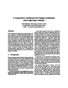
2. RELATED WORKS Various algorithms have been proposed for target localization using image-based or other modalities. These include vehicle detection and tracking using acoustic and video sensors [5]; location estimation using video, image, and audio signals [6]; location estimation based on Received Signal Strength (RSS) [7–10]; confidence-based iterative localization [11]; and target location estimation from detection of dense sensor networks [12]. Our work differs by jointly performing both classification and localization, and validating our approach under more challenging conditions using sparsely distributed sensor nodes (e.g., 0.0025 sensors per square meter). Multilateration (see Figure 1) is a common approach used for localization using wireless sensor networks (e.g., see [13, 14]). By using measured (or estimated) distances from multiple sensors, the target position can be estimated. The location of an unknown node (or target) can be estimated based on the intersection of the distance from multiple nodes. For example, Hefeeda et al. [15] provide an approach for early detection of forest fires using multilateration. Damarla et al. [16] provide a sniper localization method using the time-difference-of-arrival (TDOA) between the muzzle blast and the shock wave using multiple single-acoustic-sensor nodes. Our work differs from these works in that we employ a probabilistic score model instead of using estimated distances from nodes, and as emphasized previously, we provide a joint framework for both localization and classification. Several works estimate the motion of a target (mainly for vehicles) from acoustic signals (e.g., see [17–19]) based on the Doppler effect. While we employ estimated dynamics from the Doppler Effect, our work differs from this earlier work in that we use both acoustic and seismic signals, and we provide not only localization but also classification. Moreover, we consider both people and vehicles. Incorporating detection of peoples makes the problem significantly more challenging. This is because humans generate very small acoustic and seismic signatures compared to vehicles. In [4], an accumulative model is proposed to combine multiple evidences over time to improve discriminability. However, this introduces an unnecessary latency. Instead, we propose an accumulative method using spatially distributed sensors for improving discriminability.

Node 4

Fig. 1: Localization using multilateration. 3. JOINT LOCALIZATION AND CLASSIFICATION FRAMEWORK In this section, we describe a joint target localization and classification framework using estimated dynamics (velocities) and multimodal data. We refer to this approach as Classification and Localization using Estimated Dynamics and Multimodal data (CLEDM). In this paper, we use acoustic and seismic sensing modalities. However, the CLEDM framework is not dependent on these modalities and we envision that it can readily be adapted to other ones. Investigating such adaptations is a useful direction for future work. CLEDM is motivated by the Doppler effect, which enables us to effectively estimate the velocity of the target that is being tracked. Using a probabilistic confidence map to assess the movement of the target using estimated velocities, we estimate the next target location. We also apply the estimated velocities to improve the performance of classification. When training, modalities that exploit the Doppler effect are required. We need the ground truth class and location of the target corresponding to each signal segment in the training dataset. CLEDM decomposes time into windows (segments) of some fixed duration ts . We use ts = 1sec in our experiments. For i = 1, 2, . . ., we denote the starting time (ts × (i − 1)) of the ith segment by ti . Let Dα,i (τ ) and Dσ,i (τ ) denote the acoustic and seismic signal, respectively, for the ith time segment (0 ≤ τ < ts ). During the training process, since ground truth target location information is given, we are able to calculate two types of dynamics: a relative speed vr and an absolute speed va . We use an x − y coordinate system to model the spatial layout of the region of interest that is monitored by the given sensor network. We assume that the origin in this coordinate system is the location of an active sensor node ν that acquires the signals Dα and Dσ . If we denote the target location relative to ν at tk by ~rk = (xk , yk ), then the following expressions can be used to determine vr and va : vr =

|~ri+1 | − |~ri | , and ts

(1)

|~ri+1 − ~ri | va = . ts

(2)

Intuitively, vr is the estimated rate of change of the distance between the target and the sensor node ν. This rate of change can be positive or negative. Similarly, va represents the absolute speed of the target, which is independent of individual sensor nodes. Now suppose that Fα,i and Fσ,i represent extracted features, such as cepstral features, from Dα,i and Dσ,i , respectively, and let Ffs,i represent the concatenation [Fα,i , Fσ,i ] of these feature vectors. In this paper, we used 50 cepstral features extracted from acoustic and seismic signals for Fα,i and Fσ,i . Then we formulate the following composite feature vector Xi for time ti : Xi = [Ffs,i , va , vr ].

2

3

! ! !

! ! !

! ! !

! ! !

! ! !

4

!"""""!"""""! ! ! !

Initial location

#

$%& $% &'( )#"

! ! !

Next location candidate (p"

!"""""!"""""!

Sensor (!"

Fig. 2: Grid map for estimating the next target location.

Node 1

Node 2

Node 3

Node 4

(3)

During the training process, we compute Xi for each time segment i of available training data. We assume that a ground truth class label Yi is available as part of the training data for each time segment i. Yi indicates whether the target is of class person (A) or vehicle (B). After computing the Xi values, we train a model H to classify between classes A and B. In our experiments, we use a support vector machine (SVM) as the model H, but the CLEDM methodology is not restricted to SVMs and can readily be adapted to use other types of models. Based on the trained model H, a real-valued classification score Γ(Xi ) can be calculated if Ffs , va , and vr are given. The score is formulated such that sgn(Γ) represents the classification decision between classes A and B, and abs(Γ) represents the classification “confidence” of the associated prediction. Here, sgn and abs represent the sign and absolute value functions, respectively. After training H, we assume that the initial target location and the neighborhood N of sensors are known to initialize the tracking component of our framework. From the current target position at time ti , we can extract Fα,i , Fσ,i from Dα,i , Dσ,i . Around the current target position, which is located at a distance of ~ri from a particular sensor, we define a grid G discrete locations that represent potential target locations at time ti+1 . This grid map is illustrated in Figure 2. For a given candidate target location p = (px , py ) at time ti+1 , we set ~ri+1 = (px , py ), and then estimate va and vb from Eq. 2 and 1, respectively. Next, using Eq. 3 and our trained model, we calculate the feature vector Xi (p; ν) for the candidate next point p and sensor ν. Then, we calculate the classification score: γ(p; ν) = Γ(Xi (p; ν)).

1

(4)

Fig. 3: Confidence maps for each node are shown on the left. The spatial accumulation of these maps are shown on the right.

We repeat this process to determine γ for all points p ∈ G. For a sensor ν, we define the class-specific score functions δA and δB over the domain G as follows: ( δA (p; ν) =

|γ(p; ν)| 0

( δB (p; ν) =

0 |γ(p; ν)|

if γ(p; ν) ≥ 0 if γ(p; ν)