A Layered-Encoding Cascade Optimization Approach to Product-Mix

IEEE TRANSACTIONS ON SYSTEMS, MAN, AND CYBERNETICS—PART A: SYSTEMS AND HUMANS, VOL. 40, NO. 1, JANUARY 2010

133

A Layered-Encoding Cascade Optimization Approach to Product-Mix Planning in High-Mix–Low-Volume Manufacturing Siew-Chin Neoh, Norhashimah Morad, Chee-Peng Lim, and Zalina Abdul Aziz

Abstract—High-mix–low-volume (HMLV) production is currently a worldwide manufacturing trend. It requires a high degree of customization in the manufacturing process to produce a wide range of products in low quantity in order to meet customers’ demand for more variety and choices of products. Such a kind of business environment has increased the conversion time and decreased the production efficiency due to frequent production changeover. In this paper, a layered-encoding cascade optimization (LECO) approach is proposed to develop an HMLV product-mix optimizer that exhibits the benefits of low conversion time, high productivity, and high equipment efficiency. Specifically, the genetic algorithm (GA) and particle swarm optimization (PSO) techniques are employed as optimizers for different decision layers in different LECO models. Each GA and PSO optimizer is studied and compared. A number of hypothetical and real data sets from a manufacturing plant are used to evaluate the performance of the proposed GA and PSO optimizers. The results indicate that, with a proper selection of the GA and PSO optimizers, the LECO approach is able to generate high-quality product-mix plans to meet the production demands in HMLV manufacturing environments. Index Terms—Genetic algorithms (GAs), multidecision optimization, particle swarm optimization (PSO), product-mix planning, high-mix–low-volume (HMLV) manufacturing.

N OMENCLATURE L IST OF N OTATIONS AC CVC c1 , c2 D DT EMO Favej Fj Ftot GA

Available capacity. Conversion capacity. Constant factors for PSO. Product demand. Down time required capacity. Evolutionary multiobjective optimization. Average objective value of objective j at generation 1. Value of objective j. Total fitness value. Genetic algorithm.

Manuscript received October 18, 2007; revised September 16, 2008. First published September 22, 2009; current version published December 16, 2009. This work was supported in part by the Malaysia National Science Fellowship and in part by the School of Electrical and Electronic Engineering and the School of Industrial Technology, University of Science—Malaysia. This paper was recommended by Associate Editor L. Gunderson. S.-C. Neoh, C.-P. Lim, and Z. Abdul Aziz are with the School of Electrical and Electronic Engineering, Universiti Sains Malaysia, 14300 Nibong Tebal, Malaysia. N. Morad is with the School of Industrial Technology, Universiti Sains Malaysia, 11800 Penang, Malaysia. Digital Object Identifier 10.1109/TSMCA.2009.2029557

GAP gbest HMLV LECO M m MG Nc Nm N mu O ob OVP P pbest Pm P mu P os PSO P xovr TC TWP UBP UC V vel w Wk λj

Unused capacity or gap between available capacity and used capacity. Best found position for all particles. High-mix–low-volume. Layered-encoding cascade optimization. Minimum production volume for a product. PSO iteration number. Maximum generation for GA. Number of products to be selected for crossover. Number of products undergoing randomly selected mutation. Number of products undergoing weekly mutation. Product occurrence. Total number of objectives. Overloaded capacity penalty. Product. Best found position for a particle. Probability for randomly selected mutation. Probability for weekly mutation. Particle position. Particle swarm optimization. Probability or rate for crossover. Total capacity. Twice continuous product-occurrence penalty. Unbalanced-workload penalty. Used capacity or capacity usage in week k. Product volume. Particle velocity. Inertia weight. Week. Weight for objective j.

I. I NTRODUCTION

P

RODUCT-MIX planning involves a decision-making process of capacity distribution among products to be generated. It involves proper allocations of the amount of product generation at each time interval in order to satisfy the demand of the predicted market and utilization of the available resources. According to [1], the quality of the managerial decision making has a significant impact on the success of most business organizations. The increase of product variety in HMLV manufacturing has increased production complexity in which rapid production changeovers cause the increase of conversion time and the

1083-4427/$26.00 © 2009 IEEE

134

IEEE TRANSACTIONS ON SYSTEMS, MAN, AND CYBERNETICS—PART A: SYSTEMS AND HUMANS, VOL. 40, NO. 1, JANUARY 2010

decrease of capacity utilization and productivity. Since productmix planning affects manufacturing efficiency and productivity, it is important to have a proper product-mix optimizer, particularly in HMLV manufacturing environments. A number of approaches have been used to optimize productmix planning. In [2], methods to identify a product-mix plan with maximized profit have been studied extensively. Theory of constraints (TOC) and linear programming (LP) are two widely used approaches in product-mix planning [3]–[5]. The TOC method is applied to the product-mix problem in two areas: scheduling [6] and master production planning [7]. In [8], TOC and LP were compared, and the differences between the TOC philosophy and the LP technique were studied. Even though TOC heuristic is easily understandable and simpler to use, LP is still a better planning tool as compared with TOC when multiple constrained resources exist [8]–[10]. In addition, it is claimed that TOC is so implicit that it is considered as an incomplete approach for product-mix planning [11]. On the other hand, Onwubolu and Mutingi [12] argued that the approaches mentioned in [8]–[11] are established not in terms of computational feasibility in solving practical reallife problems typically encountered in manufacturing firms. In [12], a GA-based TOC is used because it can find highquality solutions for both small and large problems within a reasonably small computation time. Aside from that [12], GA has been applied to product-mix planning and material-match optimization in [13]. Recently, the evolutionary-algorithm (EA) community has turned much of its attention to optimization problems in industrial engineering, resulting in a fresh body of research and applications [14]–[16]. Based on the potentials of EAs in solving complex problems, this paper investigates HMLV product-mix planning with a new EA-based LECO approach. Both GA and PSO techniques are considered in analyzing the performance of the LECO-generated models in HMLV product-mix planning. Many researchers have proposed hybridization of GA and PSO to improve the mechanism of search solutions [17]–[20]. In this paper, the performance of GA and PSO hybridization in the LECO approach is investigated. In this paper, the test process in a semiconductor manufacturing industry is studied. The semiconductor industry is chosen because it involves complex production processes and operations with advanced technologies in HMLV manufacturing. Four combinations of GA and PSO LECO models are investigated, and the results are compared with those from ordinary GA without cascade stages, as well as the current method adopted in the industry, which is simply based on predicted demands. The performance of each method toward product-mix planning is measured by its ability to minimize conversion time, prevent OVP, and achieve a balanced workload throughout a specified planning horizon. In addition, a set of hypothetical data with more products is developed to assess the performance of the methods in product-mix problems that are more complicated and of a larger scale. The increase in the number of products makes product-mix planning difficult. As such, through the hypothetical data set, the capability of the LECO approach in solving more complicated product-mix problems can be demonstrated.

II. M ULTIOBJECTIVE O PTIMIZATION Most real-world problems involve multiple objectives. When solving a multiobjective combinatorial problem, the process of decision making can either be to obtain a compromised or preferred solution or to identify all nondominated solutions. According to [14], there are two basic solutions: generating and preference-based approaches. The former is used to identify Pareto solutions, whereas the latter is used to obtain compromised or preferred solutions. If prior knowledge is not available for preference structures over objectives, generating approaches have to be adopted to generate all nondominated alternatives. Otherwise, preference-based approaches, such as weighted sum, can be used to identify a compromised or preferred solution. Preference-based approaches are more appropriate for problems involving large numbers of objectives that handle some constraints as part of the objectives that have some bias in the selection process. Researchers working in the EMO community normally prefer to use the generating approaches, e.g., nondominated sorting GA, niched Pareto GA, multiobjective GA, and strength Pareto EA. Some of the recent trends in generating or Pareto-based approaches can be found in [21]–[23]. In the case study presented in this paper, some constraints are taken as part of the objectives, such as OVP and UBP. As it is preferred to have bias toward these objectives, a preferencebased approach (i.e., weighted-sum) is chosen over generating approaches.

III. N EW LECO A PPROACH Real-world manufacturing problems are normally combinatorial in nature and involve multiple objectives. One of the applications for combinatorial optimization is the efficient allocation of scarce resources to increase productivity [14]. According to [14], it is often impossible to use simple enumeration methods to solve combinatorial problems, particularly for practical problems with realistic size. Hence, EAs have been used to deal with combinatorial explosion of such problems. Conventionally, the multidimensional-encoding structure is used to represent complicated problems that involve multidecision or multirepresentation [24], [25]. When a string-based representation is no longer enough to represent the information of a problem, the multidimensional-encoding structure is used to incorporate all required constraints and decisions into one singlesolution representation. Although multidimensional encoding is a common way of problem representation, it increases the difficulty of solution analysis when the number of dimensions is large. Furthermore, fitting a multidimensional problem into 1-D encoding entails losing of information too [26]. Therefore, a layered-encoding structure is proposed to overcome the main drawback of multidimensional-encoding problems. A layered-matrix-encoding structure consists of a number of separated layers that can be used to represent different decision outputs and objectives. Instead of using complicated multidimensional encoding, layered encoding simplifies the problem representation by analyzing different decision outputs or objectives separately. Each layer is employed as an agent that

NEOH et al.: LAYERED-ENCODING CASCADE OPTIMIZATION

Fig. 1.

135

Structure of the LECO model.

is able to communicate with other agents and therefore enhance the evaluation process when optimization takes place. If the number of dimensions in multidimensional encoding is high, it is difficult to visualize the decision outputs involved. However, using layered encoding, each decision output can easily be observed by specifying the layer that represents the decision. In addition to the simplicity in analysis and visualization, another main advantage of the layered-encoding structure is that it allows multistage cascade optimization where different optimizers can be used to optimize different decisions based on the characteristic of the decision search space [27]. In this paper, a LECO structure with a two-layered 2-D matrix is used to represent the product-mix schedule. The first layer is used to determine the selection of items for the weekly available resources, and the second layer is used to determine the volume of items that is going to be tested or generated. The LECO structure is shown in Fig. 1. Acting as an agent, each layer communicates with another to find the best decision and pass it to another layer for optimization. In order to have a clearer visualization on the proposed model, the operation of a two-layered cascade optimization model for product-mix planning is shown in Fig. 2. The LECO flow of the HMLV product-mix planning used in this paper is as follows. Step 1) First-stage initialization: Randomly initialize a population of schedules on weekly item selection. Check the feasibility of each solution (individuals in the first-layer population), and regenerate the solution if it does not satisfy the constraints. Step 2) Second-stage initialization: Based on each schedule of weekly item selection, generate a population of appropriate and feasible volume allocation for the selected items. Then, an internal optimizer is initiated to find the best representative of volume allocation (the second-layer decision) for the selected items (the first-layer decision). The best representative of volume allocation is returned to the first stage and is combined with the first-layer decision. Step 3) Individual updating: Based on the fitness of each representative from the second-layer decision, an external optimizer is used to update and create a

new generation of individuals and, at the same time, retain elitism in the population. Step 4) Iteration: Repeat Steps 2) and 3) until the termination criterion is met. In this paper, GA and PSO are used as optimizers in cascade optimization. Four combinations of GA and PSO functioning as “external optimizer–internal optimizer” are studied: GA–GA, GA–PSO, PSO–PSO, and PSO–GA. GA and PSO are switched alternatively as external and internal optimizers in order to identify a better design of the cascade model toward solving the product-mix problem. In order to have a fair comparison, all combinations of the cascade model used the same population size and maximum number of generations internally and externally. Furthermore, two ordinary GA models, i.e., GA1 and GA2, are used, and the results are compared with those from the proposed model. GA1 assumes the same population size and number of generations as other cascade models, while GA2 assumes a larger population size and number of generations. Two HMLV product-mix problems with different sizes are studied, i.e., Case 1: 33 items with a four-week planning horizon and Case 2: 100 items with a four-week planning horizon. Case 1 consists of real data collected from a semiconductor manufacturing plant. In Case 2, hypothetical data are generated to analyze the performance of each cascade model in product-mix problems that are more complicated and of a larger scale. The hypothetical problem (Case 2) is included to demonstrate the ability of the proposed LECO approach in solving more complicated product-mix problems. The capacity distribution of Case 1 (real case) consists of unbalanced workload but not OVP. As such, the hypothetical case investigates the ability of LECO in addressing the overloaded issue when only a small amount of unused capacity (GAP) is available to reallocate the workload. The hypothetical case also demonstrates the effect on the computational requirements of the LECO approach in tackling product-mix problems that are of a larger scale and of a higher degree of complexity. The results are compared with those from the product-mix planning method currently adopted in the manufacturing plant, which is directly based on predicted demands.

136

IEEE TRANSACTIONS ON SYSTEMS, MAN, AND CYBERNETICS—PART A: SYSTEMS AND HUMANS, VOL. 40, NO. 1, JANUARY 2010

Fig. 2. Flowchart of the LECO model.

IV. BASIC S TRUCTURE OF P RODUCT-M IX P LANNING Multiproduct production in HMLV industries usually involves large numbers of parameters and constraints. A two-layered 2-D matrix is employed as the representation model of the product-mix problem, as shown in Fig. 3. Note that Pi (i = 1, 2, . . . , n) represents product i, whereas Di (i = 1, 2, . . . , n) represents the demand for product i that must be fulfilled within the planning horizon. The index of planning time is denoted as Wk (k = 1, 2, . . . , t), in which it determines the time interval within the product-mix planning horizon, e.g., weekly for a month. In the proposed model, the product-mix problem is represented by randomly generated product occurrence Oik and product volume Vik , where i represents the product type and k

represents the planning-time index. As shown in the following, Oik is used to indicate whether product i is selected for production in week k  1, if product i is to be produced in week k (1) Oik = 0, if otherwise. After obtaining the product occurrence, the product volume for each particular time index (Vik ) is generated randomly by fulfilling the predicted demand and the production loading rules. V. C ONSTRAINT F ORMULATION Constraints are defined as the most limited resources that prevent a system from achieving its goal [12]. There are three

NEOH et al.: LAYERED-ENCODING CASCADE OPTIMIZATION

Fig. 3.

137

Product-mix structure in the LECO model. TABLE I P OPULATION S IZE AND THE M AXIMUM N UMBER OF G ENERATIONS FOR D IFFERENT M ODELS

As shown previously, the sum of product occurrence throughout the planning horizon has to be more than zero but less than the total of product demand (Di ) divided by the minimum production volume for product i (Mi ). If Di is zero, the sum of product occurrence should be zero because no product needs to be produced if there is no demand for it. C. Capacity Constraint Capacity constraints refer to the resource ability and availability to process a particular set of product-mix plans ACk = T Ck − DTk ,

important constraints in the proposed model: demand constraint, production loading constraint, and capacity constraint. A. Demand Constraint A product-mix plan requires each product to fulfill the demand constraint of the whole planning horizon. Therefore, the sum of the generated product volume throughout the planning horizon has to be equal to the product demand as t 

Vik = Di ,

for i = 1, 2, 3, . . . , n.

(2)

k=1

for k = 1, 2, 3, . . . , t.

(4)

Equation (4) shows that the AC in week k (ACk ) is the difference between the TC of week k (T Ck ) and the down-time capacity of that particular week DTk . Note that DTk includes all capacity used for the scheduled down time (e.g., preventive maintenance and engineering experiment) and buffer time. The capacity usage based on the generated product-mix plan has to be less than or equal to the AC in the production floor, as shown in the following: U Ck ≤ ACk .

(5)

Note that U Ck (k = 1, 2, . . . , t) is given as the capacity usage in week k based on the generated product-mix plan, whereas ACk (k = 1, 2, . . . , t) is given as the AC in week k.

B. Production Loading Constraint Each manufacturing plant has its own production loading rules to control the manufacturing process effectively. Thus, each generated product-mix plan has to fulfill the production loading constraints. In this paper, the minimum production volume per product per week is a constraint. In the proposed model, Mi (i = 1, 2, . . . , n) is used to represent the minimum production volume for product i per week, and Mi = 0 0≤

t  k=1

Oik ≤

Di , Mi

for i = 1, 2, 3, . . . , n;

Mi = 0. (3)

VI. I NTERNAL AND E XTERNAL O PTIMIZERS For every first-layer decision, it is possible to have many second-layer decisions. Therefore, it is important to find a better representative in the second-layer decision before discarding the first-layer decision. Each layer of decisions can be optimized by different optimizers. As this paper involves two decision layers, hybridization of GA and PSO can be accomplished by using one of them as internal optimizer and the other as external optimizer. The internal optimizer is used to find the best representative of the second-layer decision,

138

IEEE TRANSACTIONS ON SYSTEMS, MAN, AND CYBERNETICS—PART A: SYSTEMS AND HUMANS, VOL. 40, NO. 1, JANUARY 2010

Fig. 4. Randomly selected crossover.

Fig. 6. Fig. 5. Weekly mutation.

whereas the external optimizer is employed to fine-tune the first-layer decision. As the intention is to integrate both local and global searches in a comprehensive way, the propagation of solutions consumes more computational time. Therefore, the population size and the number of iterations of the proposed model should not be too large or too small. The former leads in a long propagation time. The latter causes the first-layer decision to be discarded without considering the second-layer decision in a comprehensive manner. Table I shows the population size and number of generations for all combinations of GA and PSO, as well as GA1 and GA2. The population size and number of generations for GA1 are the same as those in the LECO models; however, those in GA2 are different, in which a larger population size and a larger generation number are used. A. GA Operations GAs are stochastic global search and optimization methods that mimic the metaphor of natural biological evolution [28]. A GA operates on a population of potential solutions applying the principle of survival of the fittest to produce successively better approximations to a solution. In this paper, it is used to search for a better decision layer, whereby the mutation and crossover operators swap the weekly item selection or volume to allow more exploration of possible solutions. 1) Selection Function: A probabilistic selection is performed based upon the individual’s fitness such that better individuals have an increased chance of being selected. Stochastic universal sampling [29], which is a single-phase sampling algorithm with minimum spread and zero bias, is used as the selection function in the proposed model. 2) Genetic Operators: As chromosomes are represented by a 2-D matrix, randomly selected crossover is applied to the selected matrix rows. The principle of randomly selected crossover is shown in Fig. 4. The crossover probability is given

Randomly selected mutation.

as P xovr, in which each individual has P xovr chance to be selected for a crossover. For each crossover, the number of rows to be selected from a 2-D matrix (number of items or products to be selected for a crossover) is denoted as N c. In other words, N c rows that are selected from one individual are to be interexchanged with another individual to produce offspring (new individuals). Two mutation techniques are suggested in the model to introduce diversity into the population, i.e., weekly mutation and randomly selected mutation. Weekly mutation is used to swap the item selection or volume of a particular week to another week, whereas randomly selected mutation is employed to randomly regenerate the weekly item selection or volume. The probability for an individual to be selected to undergo mutation is denoted as P mu for weekly mutation and P m for randomly selected mutation. For weekly mutation, the model randomly selects first the N mu numbers of rows (products) from one matrix (one individual) and then randomly swaps the volume between two randomly selected weeks, as shown in Fig. 5. Randomly selected mutation is proposed to provide random-selection modifications, where the N m number of products (rows from the 2-D matrix) is randomly selected from one individual to regenerate the product selection and volume throughout the planning horizon, as shown in Fig. 6. In this paper, the crossover and mutation rates are selected by trial and error. The suggested setting of the genetic operators is given in Table II. B. PSO Operations PSO is a stochastic population-based approach [30]. Each potential solution (also known as a particle) searches through the problem space, refines its knowledge, and adjusts its velocity based on the social information that it gathers so that its position is updated. A 2-D matrix in the representation structure is adopted as the particle-position structure in PSO. The best found position for

NEOH et al.: LAYERED-ENCODING CASCADE OPTIMIZATION

139

TABLE II G ENETIC PARAMETER S ETTING FOR C ROSSOVER AND M UTATION

a particle is denoted as pbest, whereas the best found position for all particles is denoted as gbest   velikqm = w×velikqm−1 +c1 ×rand()× pbest−P osikqm−1   + c2 ×rand()× gbest−P osikqm−1 (6) P osikqm = P osikqm−1 +velikqm .

(7)

Equations (6) and (7) compute the velocity (velikq ) and position (P osikq ) of particle q in the dimensional search space of i × k, respectively. In the equations, m is the iteration number, w is the inertia weight, c1 and c2 are two constant factors, and rand() is a randomly generated value between zero and one. A decreasing w from the range of 0.9–0.4 is applied in this paper because it has been shown to perform well in [31] and [32]. The values of c1 and c2 are both set to two, as recommended in [33], to make the weights for the “social” and “cognition” parts to be, on average, one. C. Termination Criterion The GA and PSO operations terminate when the number of M G stated for the internal and external optimizers (Table I) is reached. The overall iterations for the GA–PSO cascade flow are set to 15 and 20 for Cases 1 and 2, respectively. In the cascade model, when the termination criterion is met, GA is used to thoroughly search the second-layer decision that best fits the proposed first-layer decision at the end of cascade optimization. The final GA search is used for the purpose of enhancing product-mix planning, aiming to suggest a better product-mix plan with a combination of decisions from both layers. VII. E VALUATION F UNCTIONS Data collected from the semiconductor industry contain preferences over objectives. As constraints such as prevention of overloaded capacity, unbalanced workload, and repeated activities are handled as part of the objectives in this paper, bias in the selection process is introduced, which leads to the use

 Objective Function = minimize

t  k=1

CV Ck +

t  k=1

Fig. 7. Example of capacity consumption of week k.

of the preference-based approach (instead of the Pareto-based approach). Weighted sum, a preference-based approach, is used for fitness evaluation. All objectives to be optimized are combined to form a single objective. The objectives include reduction of CVC, maximization of machine utilization and productivity, integration of balanced workload, reduction of overloaded capacity, and reduction of repeated activities in two consecutive weeks. Constraints that are handled as objectives are introduced as penalties, e.g., OVP, UBP, and TWP. The objective function used is found in (8), shown at the bottom of the page, where CV Ck (k = 1, 2, . . . , t) refers to the CVC for week k. This includes the hardware changing time, lot setup time, and software loading time. Minimization of CVC is needed in order to reduce the impact of rapid changeovers that often occur in HMLV manufacturing environments GAPk = ACk − U Ck ,

for k = 1, 2, 3 . . . , t.

(9)

Equation (9) defines the unused capacity, or gap, for week k, where ACk and U Ck are the AC and UC in week k, respectively. The smaller the GAPk , the more utilized the resource. In this paper, a four-week capacity distribution is studied, i.e., t = 4. Note that GAPt (GAP4 ) is incorporated in the product-mix fitness evaluation so as to bring forward the workload of the fourth week. The reason of having GAP4 is to increase productivity and resource utilization in the first three weeks. Moreover, having more AC in week 4 allows production planning to incorporate more future workload to be accomplished in week 4. Thus, the objective function aims to maximize GAPt (GAP4 ) in order to bring forward the required workload to the first three weeks. The purpose of doing so is to achieve better resource utilization and to promote higher productivity in previous weeks where GAPk (k = 1, 2, . . . , t − 1)

OV Pk +

t−1  k=1

U BPk − GAPt +

n  t−1  i=1 k=1

 T W Pik

(8)

140

IEEE TRANSACTIONS ON SYSTEMS, MAN, AND CYBERNETICS—PART A: SYSTEMS AND HUMANS, VOL. 40, NO. 1, JANUARY 2010

product i is selected to be produced or tested in two weeks consecutively, T W Pik is given to product i ⎧ k+1

⎪ ⎪ Oik > 1 ⎨ 5, if k T W Pik = k+1

⎪ ⎪ ⎩ 0, if Oik ≤ 1, k

i = 1, 2, . . . , n;

k = 1, 2, . . . , t − 1.

(12)

Equation (12) shows the penalty value of T W Pik . As T W Pik considers a two-week duration at a time, k ends at t − 1 instead of t. Note that the penalty value for T W Pik is based on the preference of the manufacturing specialist. VIII. N ORMALIZATION OF THE O BJECTIVE F UNCTION

Fig. 8. Use of the U BPk function to provide a balanced workload.

is minimized. An illustration on the weekly capacity consumption and the relationship between U Ck , ACk , and GAPk is shown in Fig. 7. Note that, in (8), a negative term is introduced to GAPt for maximization purposes because the weighted-sum approach is used to minimize the overall objective function. OV Pk (k = 1, 2, . . . , t) is a penalty function associated with overloading of the weekly resource capacity for week k. It indicates that the production floor is no longer capable of fulfilling the weekly demand based on the available resource capacity. In other words, OV Pk is given when U Ck is more than ACk , as shown in the following:  100, if U Ck > ACk for k = 1, 2, 3 . . . , t. OV Pk = 0, if otherwise, (10) On the other hand, U BPk (k = 1, 2, . . . , t) is a penalty function for unbalanced workload. While GAP4 is maximized to allow higher resource utilization in the first three weeks, U BPk is introduced to minimize the variation of GAP1 , GAP2 , and GAP3 . As shown in Fig. 8, assuming that both samples consist of the same TC consumption, it can be observed that the product-mix distributions in sample I is not as systematically planned as in sample II, i.e., without U BPk , resource utilization may be too high in week 1 but too low in week 2. Therefore, it is important to introduce UBP into the proposed model. Whenever the difference between GAPk and the average of total GAPk is more than or equal to y% (which is set to 5% in this paper) of the average GAPk , U BPk is introduced to week k as follows: when U Ck > 0, for k = 1, 2, 3 . . . , t ⎛ t ⎞ ⎧ t

⎪ GAPk ⎪ ⎪ ⎜ GAPk ⎟ ⎨ GAPk − k=1 ≥ y ⎜ k=1 ⎟ 50, if t t 100 ⎝ ⎠ U BPk = ⎪ ⎪ ⎪ ⎩ 0, if otherwise. (11) In addition to OV Pk and U BPk , T W Pik (i = 1, 2, . . . , n; k = 1, 2, . . . , t − 1) is another penalty function that is introduced to reduce repeated activities in two consecutive weeks throughout the planning horizon. For instance, if

The normalization method used for the objective function in this paper is similar to the one proposed in [34] Ftot = λj

ob  Fj F j=1 avej

(13)

where Favej average objective value of objective j at generation 1; value of objective j; Fj total fitness value; Ftot weight for objective j; λj ob total number of objectives. Equation (13) shows the total normalized objective value for the evaluation function, which is calculated based on the relative fitness of the individuals with respect to the same objective. In this paper, OVP is the most important objective function, whereby a product-mix plan with OVP can ruin the whole production. Thus, OVP is given the highest weight (λ = 3). UBP is the second important objective function (λ = 2) that can affect a proper planning of capacity utilization. Unbalanced workload takes up the AC that can actually be used to increase productivity or to reduce the risk of unscheduled down time. Hence, zero OVP and UBP are the basic requirements for acceptable product-mix plans in this paper. The accepted product-mix plans can be further categorized into two groups: promising product-mix plans and high-quality product-mix plans. A promising product-mix plan does not bring forward all products in the final week, whereas a highquality product-mix plan brings forward all the final-week workload. Other than OVP and UBP, other objectives, i.e., TWP, CVC, and GAP, are given the same weight (λ = 1). Based on the aforementioned rationale, all λ settings in this paper are obtained from the experience (subjective evaluation on preference toward prevention of OVP and unbalanced capacity) of manufacturing specialists in the manufacturing plant. As five objectives are considered in this paper, the normalized evaluation function is given as Ftotp =

CV Ctotp OV Ptotp U BPtotp +3 +2 CV Cave OV Pave U BPave GAPtp T W Ptotp − + GAPave T W Pave

(14)

NEOH et al.: LAYERED-ENCODING CASCADE OPTIMIZATION

141

TABLE III O RIGINAL C APACITY D ISTRIBUTION AND P ERFORMANCE A NALYSIS FOR C ASES 1 AND 2

Fig. 9. Original capacity distribution. (a) Case 1. (b) Case 2.

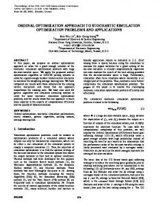
where Ftotp is the total fitness value for individual or chromosome p and CV Ctotp , OV Ptotp , U BPtotp , GAPtp , and T W Ptotp are the total CVC, the total overloaded penalty, the total UBP, the unused capacity in the final week (week t), and the total repeated-activity penalty of individual or chromosome p, respectively. On the other hand, CV Cave , OV Pave , U BPave , GAPave , and T W Pave are the average CVC, the average overloaded penalty, the average UBP, the average unused capacity in week t, and the average repeated-activity penalty of all generated chromosomes or individuals at generation 1. IX. R ESULTS AND D ISCUSSION This paper studies two product-mix plans with different sizes: 33 items with four-week planning (Case 1) and 100 items with four-week planning (Case 2). Data for Case 1 are collected directly from a semiconductor manufacturing plant, whereas data for Case 2 are generated hypothetically. The reason of using Case 2 is to expand the problem size and to evaluate the effectiveness of the proposed LECO model with different capacity-distribution scenario, e.g., how to rearrange a product-mix plan that originally contains OVP and unbalanced workload. In this paper, two machines are available for product-mix planning, and all capacity consumption is calculated as unit per machine. For example, if CVC is given as 1.2, it means that the conversion process consumes the capacity of 1.2 machine. Originally, the scheduled down time DT is fixed at 0.25 ma-

chine per week, which means that a TC of a quarter machine is not available for product-mix planning. Therefore, when GAP4 is obtained as 1.75, it means that 1.75 AC in week 4 has been made available, and no product is selected for processing or testing in week 4. In other words, all products in week 4 are brought forward to be tested in earlier weeks. Table III shows the original capacity distribution for both cases. A graphical illustration of the original capacity distribution is shown in Fig. 9. For Case 1, the original product-mix plan has a UBP of 150, indicating the existence of unbalanced workload in the original product-mix plan (Table III). This information can easily be observed from the graphical capacity distribution in Fig. 9(a). On the other hand, with U BP = 150 and OV P = 200 in Case 2, it is observed that the original product-mix plan based on the hypothetical data set consists of unbalanced workload and OVP [Table III and Fig. 9(b)]. In Fig. 9(b), the capacity percentage in week 2 exceeds 100%. This indicates that the required capacity in week 2 is more than AC, causing OVP for production in that particular week. Tables IV and V show a performance comparison and the product-mix quality of all tested approaches for both cases. A total of 30 runs have been conducted to produce the average result of each model. A. Case 1 From Table IV, all developed models have zero OVP. However, only GA1, GA2, and GA–PSO have zero UBP. This means that all product-mix plans generated by GA1, GA2, and GA–PSO are acceptable. However, for GA1, which consists of the same population size as other cascade models, none of the 30 samples gives a product-mix plan with “GAP4 = 1.75.” This indicates that all product-mix plans generated by GA1 are promising but not of high quality (Table III). In contrast, GA2 and GA–PSO gives 30 high-quality product-mix plans as the number of occurrence of “GAP4 = 1.75” is 30 out of 30 runs. Although GA2 is able to produce high-quality product-mix plans, the average CVC and TC requirement (TotReq) is higher

142

IEEE TRANSACTIONS ON SYSTEMS, MAN, AND CYBERNETICS—PART A: SYSTEMS AND HUMANS, VOL. 40, NO. 1, JANUARY 2010

TABLE IV P ERFORMANCE C OMPARISON FOR A LL D IFFERENT M ODELS IN C ASES 1 AND 2

TABLE V P RODUCT-M IX Q UALITY FOR D IFFERENT M ODELS

than those from GA–PSO. As such, GA–PSO is considered the best approach in solving Case 1 with a problem size of 33 × 4. B. Case 2 Referring to Table IV, GA1 and GA–GA have the highest probabilities of getting OVP (23 out of 30 samples). In addition, both approaches produce mostly unbalanced-workload

product-mix plans (25 out 30 samples for GA1 and 28 out of 30 samples for GA–GA). Among all approaches, GA–PSO has the lowest occurrence of OVP and UBP. For GA2, even though it is able to bring forward the final-week workload (30 out of 30 samples with GAP4 = 1.75), the higher occurrences of UBP as compared with those of GA–PSO leads to more unacceptable product-mix plans. Table V shows that the numbers of acceptable product-mix plans are 12 for GA2 and 22 for

NEOH et al.: LAYERED-ENCODING CASCADE OPTIMIZATION

143

Fig. 10. Most probable capacity distribution of Case 1 in different models.

GA–PSO. Although the number of high-quality product-mix plans in GA2 is slightly more than that of GA–PSO, the total acceptable product-mix plans is very much less than those of GA–PSO. Out of 22 acceptable product-mix plans in GA–PSO, 11 are of high quality, and 11 are considered promising. From the averages of 30 runs, GA–PSO has slightly more CVC than GA2. However, this does not imply that GA2 is better as the number of acceptable product-mix plans is very much less than that of GA–PSO. In addition, GA–PSO performs better in terms of computational time. Again, for a problem size of 100 × 4, GA–PSO is the best approach compared with other combination of cascade models, as well as the ordinary GA models that do not perform optimization by using the layered approach. C. Most Probable Capacity Distribution Throughout the 30 product-mix samples from all models in Table V, the most probable capacity distribution of each model in each case is shown in Figs. 10 and 11. The term “most probable” indicates solutions (out of the 30 samples) that occur most frequently, as given by each model. In Fig. 10, it is shown that GA1, GA–GA, PSO–GA, and PSO–PSO generate mostly promising product-mix plans in Case 1. However, they do not bring forward the workload in the final week. GA2 and GA–PSO perform better, in which all workloads in the final

week are shifted to the first three weeks. Even though both GA2 and GA–PSO give all product-mix plans that are of high quality for Case 1 (Table V), Fig. 10 shows that the TC consumption for the first three weeks in GA–PSO is less than that in GA2. As a result, GA–PSO yields better capacity distribution than GA2. By referring to Case 2 in Table V, it is observed that all models except GA–PSO have less than 50% chances of getting acceptable product-mix plans. Considering Fig. 11 for the most probable capacity distribution, GA1 and GA–GA generate mostly OVP (capacity requirement exceeds 100% of AC), whereas GA2, PSO–GA, and PSO–PSO produce mostly unbalanced-capacity distribution. As for GA–PSO, there are two most probable capacity distributions because, out of 22 accepted product-mix plans, 11 of them are promising, and the others are of high quality (Table V). Overall, GA–PSO is the best cascade optimization model in this paper. It outperforms the ordinary GAs (GA1 and GA2) in TC consumption and provides more acceptable product-mix plans. GA2, which has a larger population size, has less occurrence of TWP as compared with that of GA–PSO. However, it is still inferior to GA–PSO in the overall performance. In terms of computational time and maximum number of generations (M G), if GA–PSO is allowed to run for a longer period, or a larger M G is used, the occurrence of TWP in GA–PSO can be reduced.

144

IEEE TRANSACTIONS ON SYSTEMS, MAN, AND CYBERNETICS—PART A: SYSTEMS AND HUMANS, VOL. 40, NO. 1, JANUARY 2010

Fig. 11. Most probable capacity distribution of Case 2 in different models.

D. Improvement

E. Computational Time

Table VI shows the percentage of improvement brought by all developed models (based on the most probable product-mix distributions) in comparison with the original product-mix performance. It is clearly shown that all models give improvement in CVC, OVP, GAP, and UBP for both cases. GA–PSO is the best in overall improvement, whereas other cascade models do not perform well in terms of TWP in Case 2. The percentage of improvement given by GA–PSO for CVC is the highest: 45.78% in Case 1 and 35.42% in Case 2. Even though GA1 and GA2 exhibit improvements, they are inferior to GA–PSO.

As expected, Case 2 consumes higher computational times than Case 1. The increase in the number of products or variables in HMLV problems has a significant effect on the required computational time. While GA–GA, PSO–GA, and PSO–PSO require higher computational times as compared with GA2, GA–PSO consumes lower computational time than GA2. Therefore, selecting appropriate internal and external optimizers in the LECO model is important to reduce computational overhead. It is undeniable that adding more variables in HMLV problems leads to an increase in computational complexity. However, with an appropriate selection of

NEOH et al.: LAYERED-ENCODING CASCADE OPTIMIZATION

145

TABLE VI I MPROVEMENTS F ROM THE O RIGINAL P RODUCT-M IX P LANS ACHIEVED BY D IFFERENT M ODELS

optimizers and with advances in computing hardware and software nowadays, the computational complexity can be mitigated, e.g., GA–PSO uses less than 44 min on average to yield its solution in the complicated hypothetical case. X. C ONCLUSION In this paper, a LECO model has been introduced as an optimization approach to solving HMLV product-mix problems. The LECO structure has been suggested to enhance the solution of multilayer-decision optimization tasks. Different combinations of internal and external optimizers using GA and PSO have been developed to find the best LECO model. Combining appropriate optimizers lead to better local and global searches. Among all developed models, GA–PSO is the best candidate in this paper. Theoretically, GA is well known for performing global search, whereas PSO is widely accepted for its ability to learn from social behaviors. The combination of GA–PSO has allowed both global and local searches to be carried out effectively. Ordinary GAs with different population size and number of MG have also been developed for performance comparison with the LECO models. The results show that GA–PSO is able to outperform the ordinary GAs in generating high-quality product-mix plans. When a larger scale problem is used, it could save up to nearly 50% of the computational time as compared with that of the ordinary GAs. In short, the GA–PSO model is a useful alternative tool for tackling HMLV productmix problems. A normalized weighted-sum approach is used as the fitnessevaluation function throughout this paper. For further work, Pareto-based approaches can be tested to further investigate the

applicability of the LECO approach. In addition, improvement can be carried out using different optimizers other than GA and PSO to assess the most suitable hybridization for the LECO approach. R EFERENCES [1] S. Ram, “Design and validation of a knowledge-based system for screening product innovations,” IEEE Trans. Syst., Man, Cybern. A, Syst., Humans, vol. 26, no. 2, pp. 213–221, Mar. 1996. [2] G. Buxey, “Production scheduling: Practice and theory,” Eur. J. Oper. Res., vol. 39, no. 1, pp. 17–31, Mar. 1989. [3] J. Miltenburg, “Comparing JIT, MRP and TOC, and embedding TOC into MRP,” Int. J. Prod. Res., vol. 35, no. 4, pp. 1147–1169, Apr. 1997. [4] M. C. Patterson, “The product-mix decision: A comparison of theory of constraints and labor-based management accounting,” Prod. Invent. J., vol. 33, no. 3, pp. 80–85, 1992. [5] B. Ronen and M. K. Starr, “Synchronized manufacturing as in OPT: From practice to theory,” Comput. Ind. Eng., vol. 18, no. 4, pp. 585–600, 1990. [6] E. Schragenheim, DISASTERTM Scheduling Software Teaching Material. New Haven, CT: Goldratt Inst., 1991. [7] E. M. Goldratt, The Haystack Syndrome. New York: North River, 1990. [8] R. Luebbe and B. Finch, “Theory of constraints and linear programming: A comparison,” Int. J. Prod. Res., vol. 30, no. 6, pp. 1471–1478, Jun. 1992. [9] T. N. Lee and G. Plenert, “Maximizing product-mix profitability—What’s the best analysis tool,” Prod. Plan. Control, vol. 7, no. 6, pp. 547–553, 1996. [10] G. Plenert, “Optimization theory of constraints when multiple constrained resources exist,” Eur. J. Oper. Res., vol. 70, no. 1, pp. 126–133, Oct. 1993. [11] T. C. Hsu and S. H. Chung, “The TOC-based algorithm for solving product mix problems,” Prod. Plan. Control, vol. 9, no. 1, pp. 36–46, 1998. [12] G. C. Onwubolu and M. Mutingi, “Optimizing the multiple constrained resources product mix problem using genetic algorithms,” Int. J. Prod. Res., vol. 39, no. 9, pp. 1897–1910, Jun. 2001. [13] S. A. Ali, R. de Souza, and H. Zahid, “Intelligent product-mix and material match in electronics manufacturing,” Neural Parallel Sci. Comput., vol. 11, no. 1/2, pp. 97–118, Mar. 2003. [14] M. Gen and R. Cheng, Genetic Algorithms and Engineering Optimization. New York: Wiley, 2000.

146

IEEE TRANSACTIONS ON SYSTEMS, MAN, AND CYBERNETICS—PART A: SYSTEMS AND HUMANS, VOL. 40, NO. 1, JANUARY 2010

[15] S. Y. Ho, H. S. Lin, W. H. Liauh, and S. J. Ho, “OPSO: Orthogonal particle swarm optimization and its application to task assignment problems,” IEEE Trans. Syst., Man, Cybern. A, Syst., Humans, vol. 38, no. 2, pp. 288– 298, Mar. 2008. [16] G. S. Tewolde and W. Sheng, “Robot path integration in manufacturing processes: Genetic algorithms versus ant colony optimization,” IEEE Trans. Syst., Man, Cybern. A, Syst., Humans, vol. 38, no. 2, pp. 278–287, Mar. 2008. [17] M. Settles and T. Soule, “Breeding swarms: A GA/PSO hybrid,” in Proc. Conf. Genetic Evol. Comput., 2005, pp. 161–168. [18] A. Gandelli, F. Grimaccia, M. Mussetta, P. Pirinoli, and R. E. Zich, “Genetical swarm optimization: An evolutionary algorithm for antenna design,” J. Automatika, vol. 47, no. 3/4, pp. 105–112, 2006. [19] Y. Kao and E. Zahara, “A hybrid genetic algorithm and particle swarm optimization for multimodal functions,” Appl. Soft Comput., vol. 8, no. 2, pp. 849–857, Mar. 2008. [20] H. Shi, Y. C. Liang, H. P. Lee, C. Lu, and L. M. Wang, “An improved GA and a novel PSO–GA-based hybrid algorithm,” Inf. Process. Lett., vol. 93, no. 5, pp. 255–261, Mar. 2005. [21] C. A. C. Coello, “A comprehensive survey of evolutionary-based multiobjective optimization techniques,” Knowl. Inf. Syst., vol. 1, pp. 269–308, 1999. [22] C. A. C. Coello, “Recent trends in evolutionary multiobjective optimization,” in Evolutionary Multiobjective Optimization: Theoretical Advances & Applications. London, U.K.: Springer-Verlag, 2005, pp. 7–32. [23] E. Zitzler and L. Thiele, “Multiobjective evolutionary algorithms: A comparative case study and the strength Pareto approach,” IEEE Trans. Evol. Comput., vol. 3, no. 4, pp. 257–271, Nov. 1999. [24] C. J. Huang, C. Chen, C. S. Chou, and S. T. Kao, “Fast packet classification using multi-dimensional encoding,” in Proc. HPSR Workshop, 2007, pp. 1–6. [25] G. A. Vignaux and Z. Michalewicz, “A genetic algorithm for the linear transportation problem,” IEEE Trans. Syst., Man, Cybern., vol. 21, no. 2, pp. 445–452, Mar./Apr. 1991. [26] T. N. Bui and B. R. Moon, “On multi-dimensional encoding/crossover,” in Proc. 6th Int. Conf. Genetic Algorithms, 1995, pp. 49–56. [27] S. C. Neoh, A. Marzuki, N. Morad, C. P. Lim, and Z. Abdul Aziz, “An interactive genetic algorithm approach to MMIC low noise amplifier design using a layered encoding structure,” in Proc. IEEE WCCI, Hong Kong, Jun. 1–6, 2008, pp. 1571–1575. [28] J. Holland, Adaptation in Natural and Artificial Systems. Ann Arbor, MI: Univ. Michigan Press, 1975. [29] H. K. Yii, “Development of a neuro-genetic based hybrid framework for the solder paste printing process,” M.S. thesis, Univ. Sains Malaysia, Penang, Malaysia, 2001. [30] N. P. Padhy, Artificial Intelligence and Intelligent Systems. London, U.K.: Oxford Univ. Press, 2005. [31] S. Naka, T. Genji, T. Yura, and Y. Fukuyama, “A hybrid particle swarm optimization for distribution state estimation,” IEEE Trans. Power Syst., vol. 18, no. 1, pp. 60–68, Feb. 2003. [32] H. Yoshida, K. Kawata, Y. Fukuyama, S. Takayama, and Y. Nakanishi, “A particle swarm optimization for reactive power and voltage control considering voltage security assessment,” IEEE Trans. Power Syst., vol. 15, no. 4, pp. 1232–1239, Nov. 2000. [33] J. Kennedy and R. Eberhart, “Particle swarm optimization,” in Proc. IEEE Int. Conf. Neural Netw., 1995, pp. 1942–1948. [34] N. Morad, “Optimization of cellular manufacturing systems using genetic algorithms,” Ph.D. dissertation, Univ. Sheffield, Sheffield, U.K., 1997.

Siew-Chin Neoh received the B.S. degree in quality control and instrumentation from the School of Industrial Technology, Universiti Sains Malaysia (USM), Penang, Malaysia. She is currently working toward the Ph.D. degree in the School of Electrical and Electronic Engineering, USM, Nibong Tebal. Her research interests include production planning and optimization, intelligent manufacturing systems, evolutionary computing, operations management, and decision support systems.

Norhashimah Morad received the B.Sc. degree in chemical engineering from the University of Missouri, Columbia, in 1985 and the Ph.D. degree in control engineering from the University of Sheffield, Sheffield, U.K., in 1997. Her current research interests are in the development of intelligent systems (using artificial neural networks and genetic algorithms), life-cycle assessment, and treatment of wastewater. She is currently an Associate Professor with the School of Industrial Technology, Universiti Sains Malaysia, Penang, Malaysia.

Chee-Peng Lim received the B.Eng. (electrical) degree from the Universiti Teknologi Malaysia, Skudai, Malaysia, in 1992 and the M.Sc. (control systems) and Ph.D. degrees from the University of Sheffield, Sheffield, U.K., in 1993 and 1997, respectively. He is currently a Professor with the School of Electrical and Electronic Engineering, Universiti Sains Malaysia, Nibong Tebal, Malaysia. He has published more than 150 technical papers in books, international journals, and conference proceedings. His research interests include soft computing, pattern recognition, medical prognosis and diagnosis, fault detection and diagnosis, and condition monitoring.

Zalina Abdul Aziz received the Ph.D. degree in quality engineering from Newcastle University, Newcastle upon Tyne, U.K., and the M.Sc. and B.B.A. degrees in applied statistics from Western Michigan University, Kalamazoo. She is currently an Associate Professor with the School of Electrical and Electronic Engineering, Universiti Sains Malaysia (USM), Nibong Tebal, Malaysia. Over the past 16 years, she has been promoting the use of quality-engineering techniques to manufacturing industries in Malaysia, collaborating with them on the implementation of techniques, and providing solutions to the problems that arise during the implementation process. One of the techniques that is of special interest to her is the “design of experiments” technique.