reduces the network overhead produced by heartbeat-style failure detectors. ... no such message, the answer is âno suspectâ, but a ping is sent to verify this ...
The Third International Conference on Availability, Reliability and Security
A Lazy Monitoring Approach for Heartbeat-Style Failure Detectors Benjamin Satzger, Andreas Pietzowski, Wolfgang Trumler, and Theo Ungerer Institute of Computer Science, University of Augsburg D-86135 Augsburg, Germany Email: {satzger, pietzowski, trumler, ungerer}@informatik.uni-augsburg.de Abstract—Failure detectors are a fundamental part of safe fault-tolerant distributed systems. Many failure detectors use heartbeats to draw conclusions about the state of nodes within a distributed environment. The contribution of this paper is an approach whose benefits are twofold. On the one hand it reduces the network overhead produced by heartbeat-style failure detectors. On the other hand it improves the quality of these failure detectors by providing them with richer information about the current network condition. We call this approach lazy monitoring since the active sending of heartbeats is avoided if possible. As it is independent of the actual failure detection algorithm it can be used in many domains. For evaluation purposes we applied our approach to the Smart Doorplate Project. In this testbed the proposed technique reduced the traffic to 1.2% while providing much more information about the environment to the failure detectors.
I. I NTRODUCTION Failure detectors are an important part of fault-tolerant distributed systems and are thus widely used. They provide information on failures of components of these systems. While the research focus so far has been on improving the quality of the failure detection algorithms this work aims at reducing their overhead and prividing them with more information about the distributed system. Dependant on the used failure detection algorithm more information about the environment should also improve the detection quality. The proposed lazy monitoring approach can be used in combination with an important subset of failure detectors called push or heartbeat-style failure detectors. There exist two main monitoring approaches for failure detectors: push and pull. Assuming there are two nodes or processes p and q where p has a failure detector monitoring q. Using a push failure detector q has to send heartbeat messages to p. This information is used by p to draw conclusions about q’s status. A very simple failure detection algorithm using the push approach works as follows: q sends heartbeat messages at regular time intervals ∆i to p. When p receives a heartbeat message it trusts q for a certain period of time ∆to . If this period elapses without receiving a newer heartbeat, p starts to suspect q. Due to the use of heartbeat messages, failure detectors that are based on a push mechanism are also called heartbeat-style failure detectors. Many state-of-the-art algorithms are based on heartbeats, see e.g. [1], [2], [3], [4]. In systems with a pull failure detection the monitored node
0-7695-3102-4/08 $25.00 © 2008 IEEE DOI 10.1109/ARES.2008.51
adopts a passive role. p monitors q by sending “are you still alive”-messages every ∆i . If p does not receive an answer from q within a certain period of time ∆to , p is suspecting q. Failure detectors using the push paradigm have some benefits compared to pull failure detectors. They need only half the messages for an equivalent failure detection quality. Furthermore it is harder to determine the timeout ∆to as two messages need to be taken into account which are both sent over the network and subject to network delays and loss, while in push failure detectors only one message has to be considered. We define a heartbeat-style failure detector to be lazy if it applies a technique to reduce the networking overhead that arises from sending heartbeat messages. The analogy is that these algorithms only send heartbeat messages if they really have to and are thus called lazy. In this context it is important to distinct application messages from heartbeat messages. The former are sent by the application and cannot be avoided, heartbeat messages are sent by failure detectors. Fetzer et al. [5] introduced the term lazy failure detector but came up with a slightly different definition which does not fit to heartbeat-style failure detectors very well. Their algorithm requires that each application message is being acknowledged. Thus the round trip delay of each application message together with its acknowlegement message is calculated. In addition, for each destination the maximum round trip delay is stored. The output of the failure detector depends on the existence of a pending message, i.e. a message such that the application message has been sent but not acknowledged yet: If there is no such message, the answer is “no suspect”, but a ping is sent to verify this answer. If there is such a message, the answer depends on the maximum round trip delay. The lazy monitoring approach proposed in this work also uses application messages in order to save overhead, but has some noteworthy features in comparison to the failure detector of [5]. The usage of application messages in order to save overhead is an integrated part of the failure detector of Fetzer et al. and is not applicable to other failure detection algorithms. Our lazy monitoring approach can be seen as a form of a plugin that can be used with heartbeat-style failure detectors. Fetzer’s algorithm uses application messages and is thus able to save in the optimal case 50% of its message overhead. It is based on computing round trip delays. Instead of sending ping-pong messages, with the use of application messages
404
Authorized licensed use limited to: University Augsburg. Downloaded on October 26, 2009 at 18:54 from IEEE Xplore. Restrictions apply.
12 10 8 6
Frequency
4 2
II. FAILURE DETECTION ALGORITHMS As system model two processes p and q are considered which are connected by a communication channel. They can only communicate by sending and receiving messages. Furthermore it is assumed that each process has access to a local clock that is able to measure time intervals whereas the clocks are not synchronised. As in the previous section, suppose that process p is monitoring q using a heartbeatstyle failure detector. Thus q sends heartbeat messages to p while p uses them to draw conclusions about q’s status. Process p manages a sample base S where it stores these information. This sample base typically consists of inter-arrival times of received heartbeats. Some algorithms do not use inter-arrival times but absolute arrival times of heartbeats. As a transformation from the inter-arrival times to the absolute times is easily possible, in the following it is assumed that the sample base S consists of the former. Along with S, p also stores the selected heartbeat period ∆i , i.e. the interval q sends hearbeat messages to p, and the freshness point f , i.e. the time when the last heartbeat was received. At runtime, p could for instance have the following relevant information: • S = [1.083s, 0.968s, 1.062s, 0.993s, 0.942s, 2.037s, . . .] • ∆i = 1 second • f = 2007-10-22 10:06:02.434 (local clock) • current time: 2007-10-22 10:06:02.919 (local clock) Based on this data failure detectors generate a suspicion value which indicates whether q has failed or not. Failure detectors differ in the way the suspicion value is computed but they all are dependant on the input from the sample base S. Chen et al. [2] propose a well-known adaptive failure
detection approach based on a probabilistic analysis. The algorithm uses the sample base to compute an estimation of the arrival time of the next heartbeat. The timeout is set according to this estimation plus a constant safety margin. Bertier et al. [3] combine Chen’s estimation with another estimation developed by Jacobson [7] for a different context. Their approach is similar to Chen’s - however they do not use a constant safety margin but compute it with Jacobson’s algorithm. Hayashibara et al. [4] propose a so-called ϕ failure detector that is based on an estimation of inter-arrival times in the sample base assuming that inter-arrivals follow a normal distribution. In contrast to the previous two failure detectors this failure detector is accrual as it does not output whether a process is suspected to have crashed or not. Rather it gives a suspicion information on a continuous scale whereas higher values indicate a higher probability that the monitored process has failed. Satzger et al. [1], [8] also introduce an accrual failure detector based on a statistical analysis of the samples but do not assume the inter-arrival times to follow a certain probability distribution. Each of these four exemplary cited adaptive heartbeat-style failure detectors can be combined with the lazy monitoring approach presented in the next section. Before, the failure detector of Satzger et al. is presented in more detail to provide an impression of the functionality of failure detection algorithms. Suppose q sends heartbeat messages to p at a heartbeat interval ∆i = 1 second. Process p manages a list S with information about the inter-arrival times of the last n heartbeats it received. Let us assume S = [1.083s, 0.968s, 1.062s, 0.993s, 0.942s, 2.037s, 0.872s, . . .] at a certain point during runtime. The variations of the times in S are due to the variations of the network sending delays and also message losses. Furthermore p stores the time of the last received heartbeat called freshness point f . Based on the sampled inter-arrival times in S and f the failure detection algorithm estimates the probability that no further heartbeat messages arrive, i.e. q has failed. Figure 1 shows the values of S as a histogram. The shape of the histogram of S depends
0
it is able to save the “ping”-fraction. Our lazy monitoring concept is capable of saving nearly all the overhead produced by heartbeat-style failure detectors. Larrea et al. [6] also have made contributions to improve the communication efficiency of failure detectors. They assume a network of n processes forming a ring while the processes send heartbeats to their successor and monitor their predecessor by listening for heartbeats. Their focus is on reducing the number of unidirectional links between processes that carry messages forever. The authors of [6] also propose to piggyback information, more precisely to append a suspicion list to sent heartbeats. By contrast we want to save the heartbeats themselves and do not piggyback possibly large data like a list. This paper aims at using application messages as alive proof which is not novel. But so far, this fundamental concept cannot be used together with heartbeat-style failure detectors. These failure detectors completeley depend on heartbeats sent at regular intervals and are incapable exploiting information application messages are providing about the environment. The main contribution of this paper is to close this gap. In the following Section II, some heartbeat-style failure detectors are presented to convey how these algorithms work. In Section III the proposed lazy monitoring approach is introduced. Section V provides an evaluation and finally, Section VI concludes the paper.
1.0
1.5
2.0
2.5
3.0
3.5
4.0
time in seconds
Fig. 1.
Histogram of the sampled inter-arrival times in S
on ∆i and the communication channel connecting q and p. In our example ∆i is one second. The communication channel has a message loss rate of 10% and a certain fluctuating
405
Authorized licensed use limited to: University Augsburg. Downloaded on October 26, 2009 at 18:54 from IEEE Xplore. Restrictions apply.
0.6 0.4 0.0
0.2
Cumulative frequency
0.8
1.0
message sending delay. The peak at two seconds arises from one lost heartbeat message, the peak at three seconds arises from two consecutive lost heartbeat messages, and so forth. Figure 2 shows the cumulative frequencies of the values in S. These cumulative frequencies are used by the failure detection algorithm to compute a suspicion value for the failure of q. If p is for example waiting since two seconds for the next heartbeat of q in this example the failure probability is about 95%. This procedure is graphically depicted with arrows within Figure 2. As you can see the inter-arrival times in S are
1
2
3
4
time in seconds
Fig. 2.
Cumulative frequencies of the sampled inter-arrival times in S.
the determining factor for the output of the failure detector. S contains information about how the heartbeat messages behaved in the past. This knowledge allows for an estimation of the current state of q. In the next section the lazy monitoring approach is introduced that allows to save overhead using failure detectors like the ones introduced here. III. L AZY MONITORING APPROACH Failure detectors should send as few messages as possible. There are two ways to influence the amount of sent heartbeat messages. First, heartbeat-style failure detectors are tailorable, what denotes the ability to downgrade the detection quality for the benefit of a lower network load. The heartbeat interval ∆i is the key to tailor the failure detector in this way: A small heartbeat interval results in a high network load, but failures can be detected rapidly. Figure 3 shows the traditional sampling method for the heartbeat inter-arrival times. The monitored process q sends heartbeat messages to the monitoring process p every ∆i . Process p manages a list S - the sample base with the sampled inter-arrival times - along with the freshness point f which is always set to the time when the last heartbeat was received and the heartbeat interval ∆i . This information is needed by most failure detectors to compute a suspicion value. Whenever p receives a heartbeat, it appends s = tr − f (tr is the current time) to S and sets f = tr afterwards. Most failure detectors limit the size of S to a certain value n (e.g. n = 1000) causing the oldest sample being deleted if a new one is inserted into S.
Process q: send heartbeat message to p every ∆i Process p: f = −1 //freshness point S = nil //S is initialised as an empty list upon receive heartbeat message mj at time tr if f == -1 then f = tr else s = tr − f ; f = tr ; append s to S Fig. 3.
endif
Traditional heartbeat sampling
Our lazy monitoring approach aims at reducing the network load without the negative effects on the detection time. Quite the contrary it allows for a better training of the failure detector as it provides more data and thus can furthermore improve the quality of the generated suspicion information. Thereby we distinguish between application messages and heartbeat messages. Application messages are messages that are sent by the members of the network in the normal mode and cannot be avoided. Heartbeat messages are the messages sent by failure detectors. This work aims at avoiding the overhead of sending heartbeats by appending small amounts of data to the application messages. First, it is assumed that application messages behave the same way as heartbeat messages. Limitations of this generalisation are discussed below. Friedman et al. [9] compare the throughput and latency of four protocols that provide total ordering. They come to the conclusion that message packing influences the performance overwhelmingly more than any other optimization that they checked both in terms of throughput and latency. The reason is that packing messages reduces amongst others the header overhead for messages and the contention on the network. Our approach can be interpreted as some kind of message packing where the problem lies in enabling failure detectors to use them as samples. This is not possible yet for heartbeat-style failure detectors. In order to save a heartbeat message, our approach needs a consecutive id and a timestamp to be appended to an application message. In heartbeat-style failure detection algorithms q sends a heartbeat to p every ∆i seconds and p is sampling the inter-arrival times of these heartbeats. Note that the calculation of inter-arrival times is always possible, provided p has a local clock. If the lazy monitoring approach is applied, process q’s heartbeat sending behaviour must be slightly changed. A heartbeat is not sent automatically every ∆i , but q is responsible to send one to p if no message, either application or heartbeat message, has been sent to p since ∆i . Thus pure heartbeat messages are only used if no application message has been sent since ∆i . But a significant problem arises because the failure detector is now unable to compute new heartbeat inter-arrival times to insert into the sample base S. The sample base consists of heartbeat inter-arrival times which are typically around ∆i . The inter-arrival times of application messages are arbitrary and have no informative value for a failure detector. Thus, the basic issue is to provide a technique that allows
406
Authorized licensed use limited to: University Augsburg. Downloaded on October 26, 2009 at 18:54 from IEEE Xplore. Restrictions apply.
failure detectors to sample inter-arrival times although only application messages are sent at random times instead of heartbeats. Basically, the inter-arrival times S in traditional failure detectors are mainly influenced by the following three environmental circumstances: Message delay: Heartbeats sent over the network are affected by message delays. Message loss: It can occur that heartbeat messages get lost during the sending process. Processing delay of q: The monitored process q sends heartbeat messages not at the time it is supposed, e.g. due to processing overload. In many systems the variations of the inter-arrival times due to processing delays of q are negligible. Therefore, in this work, we concentrate on message delay and message loss. In the following the concept of lazy heartbeat sampling is introduced. This enables p to sample heartbeat inter-arrival times in order to adapt to the actual network conditions, even if application messages are used instead of heartbeats. By this means, the failure detector is able to adapt even faster to changing networking conditions, as application and heartbeat messages can be used to sample inter-arrival times. Due to the fact that every message is used to draw conclusions about the network’s condition a much richer set of training information is available. To realise the lazy heartbeat sampling, q is supposed to append a consecutively numbered id and the sending time according to its local clock to every message it sends to q. It is shown in the following that, with this additional information, process p can use every message it receives to compute a sample s for the sample base S. While heartbeat messages are sent every ∆i , application messages can be sent at random times. The following Formula 1 transformes the inter-arrival times of the application messages into inter-arrival times representing an estimation for heartbeats sent instead of the application messages. Thus application messages are made useful for the failure detection task. This formula is the core of this work and consists of three parts: s=
∆i ���� heartbeat interval
+
(l · ∆i ) + (∆r − ∆s ) � �� � � �� � message loss
(1)
sending time
Heartbeat interval: The heartbeat interval ∆i is the expected value for the inter-arrival times of heartbeats and the basis for the lazy heartbeat inter-arrival time estimation. Message loss: Lost messages can be identified by the piggybacked message-ids. Every consecutively lost message lengthens the estimated heartbeat inter-arrival time by ∆i . l is the number of consecutively lost messages what arises from the message-ids (l = current received message-id - last received message-id -1). Therefore l · ∆i adds the additional time by lost messages to Formula 1. Sending time: The term ∆r − ∆s reflects the variations of the inter-arrival time through the network. ∆r is the difference of the receipt times of the current message and the previously received message according to p’s local clock and ∆s is the
difference of the sending times of the current message and the previously received message according to q’s local clock what can be computed by p with the appended sending times. Figure 4 presents the lazy heartbeat sampling in detail. To Process q: - append sending time ts and consecutive id to every outgoing message - if no message has been sent to p since ∆i , send heartbeat message to p Process p: f = −1 //freshness point S = nil //S is initialised as an empty list upon receive of message mj at time tr if f == -1 then f = tr else s = tr − f ; s = ∆i + (l · ∆i ) + (∆r − ∆s ) f = tr ; append s to S endif Fig. 4.
;
Lazy heartbeat sampling
clarifiy the functionality of the new lazy monitoring approach two examples are discussed. Example 1 In this first example it is assumed that two application messages are sent within an interval that is shorter than the heartbeat interval. None of these two messages gets lost. ∆i : heartbeat interval is 1000 ms mi−1 : • message-id: i-1 • sending time: 0000 (according to q’s clock) • receipt time: 0500 (according to p’s clock) mi : • message-id: i • sending time: 0250 (according to q’s clock) • receipt time: 0800 (according to p’s clock) The messages mi−1 and mi are two application messages that are sent from q to p. The message-ids i and i − 1 indicate that no message has been lost and thus l = 0 in this case. The message mi has been sent exactly 250 ms seconds after mi−1 . The interesting point here is that the sending times have an interval of 250 ms, the receipt times of 300 ms seconds. Thus the sending time variation is 50 ms. The basic idea of this lazy monitoring approach is roughly spoken “if the application message were a heartbeat what would a sample look like”. If the values of this example are inserted into Equation 1 the result is: s = ∆i + (l · ∆i ) + (∆r − ∆s ) = 1000 ms + (0 · 1000 ms) + (300 ms − 250 ms) = 1050 ms The inter-arrival time of mi and mi−1 is 300 ms seconds - the sending interval is 250 ms. Heartbeat messages are supposed to be sent every 1000 ms. Thus if these two application messages were heartbeat messages then they would have been sent with an interval of 1000 ms and the inter-arrival time that q had experienced would be 1050 ms. Example 2 In the second example we analyse a case where one message gets lost. This can be recognised with the message-ids. ∆i : heartbeat interval is 1000 ms
407
Authorized licensed use limited to: University Augsburg. Downloaded on October 26, 2009 at 18:54 from IEEE Xplore. Restrictions apply.
mi−2 :
message-id: i-2 sending time: 0000 (according to q’s clock) • receipt time: 0300 (according to p’s clock) mi : • message-id: i • sending time: 0800 (according to q’s clock) • receipt time: 1030 (according to p’s clock) With this setting the sample s is calculated as follows: s = ∆i + (l · ∆i ) + (∆r − ∆s ) = 1000 ms + (1 · 1000 ms) + (730 ms − 800 ms) = 1930 ms In this example p sends three application messages to q whereas the second gets lost. With the same probability the loss could also have happened to a sent heartbeat message. Furthermore the sending time of mi is 70 ms shorter than the sending time of mi−2 . This example transferred to the case of real heartbeat messages would result in an inter-arrival time of 1930 ms. The meaning of Equation 1 should be clearer now: every message is used to draw conclusions about the conditions a heartbeat would undergo if sent at the same time. Process q passes on sending real heartbeat messages if application messages are sent. Process q however is still able to sample heartbeat inter-arrival times and can update its knowledge base, the list of inter-arrival times S. The failure estimation algorithm of heartbeat-style failure detectors do not have to be changed in order to apply this lazy monitoring approach. If processes are communicating frequently no single heartbeat message has to be sent and nearly no network overhead is produced by failure detectors. It is also possible to improve the quality of failure detectors by reducing the heartbeat interval ∆i . Thus failures can be detected faster - the bigger network overhead caused by this action could cease to exist with the application of our lazy monitoring approach. If no application messages are sent then of course heartbeat messages have to be used. But it can be argued that in this case there is a very low network load and the additional network load caused by heartbeat messages can be beared. However, during high traffic times where additional traffic would be very unpleasant our approach prevents the network from this overhead. It has to be mentioned that our approach introduces overhead as a message id and the sending time is appended to application messages. However, this overhead can be reduced to 4 bytes or even less per message. Suppose the message id is represented with 10 bits and the timestamp with 22 bits what together are 4 bytes. Then, the message id has a range from 1 to 1024, and a timestamp can be represented by the number of milliseconds since the last full hour. The check for lost messages as well as the delay calculation has then to be performed with modulo 210 and 222 respectively. Of course, p is now unable to distinct e.g. whether none or 1024 consecutive messages have been lost, but the latter case is very unlikely and can be ignored. The analogue is holding for the appended timestamp. • •
IV. M ESSAGE SELECTION STRATEGY In this section we address two issues. First, until now we assumed that the behaviour of application messages is
a good estimator for the behaviour of heartbeat messages. However, this is not the case if application messages can become much larger than heartbeats. One way to overcome this is to perform the piggybacking of the relevant information at packet level. But as the engineering of this heavily depends on the used protocols and often the access to these layers is neither given nor wanted we only consider lazy monitoring on the application/message level in this work. Second, in the last section lazy monitoring information is appended to all application messages - this is not always necessary. A message selection strategy determines which messages to use for lazy failure detection. This is useful to (1) omit application messages which are too large and therefore unsuitable as information source for failure detectors and (2) to adjust the amount of suitable messages which are used for lazy monitoring. A message selection strategy (MSS) takes as input an application message and outputs whether it is used for lazy monitoring, i.e. whether a message id and a timestamp is appended which can be processed at the receiving node. The simplest strategy is to omit all application messages which are larger than M AXSIZE bytes and to use the remaining ones. Application messages smaller or equal to M AXSIZE are supposed to have similar behaviour to heartbeat messages and therefore considered suitable for lazy monitoring. If all suitable application messages are used for lazy monitoring a maximum number of samples is provided to the failure detector. As some failure detectors might not be able to profit from an amount of samples higher than a certain value nu per interval ∆i also suitable application messages can be omitted to reduce overhead. Suppose ns is the average number of suitable messages within an interval ∆i and nu is the maximum number of messages the failure detector can utilise as samples. The adaptive MSS of Figure 5 reduces the number of messages used for lazy monitoring to nu on average. The function rand() returns a random value within Process q: for every outgoing message m: if sizeof (m) ≤ M AXSIZE and rand() < nnus then \\message is selected for lazy monitoring append sending time ts and consecutive id to m endif if no selected message has been sent to p since ∆i , send heartbeat message to p Fig. 5.
Adaptive MSS
the interval [0, 1). V. E VALUATION In this section we describe the costs and benefits of our approach with respect to (1) the produced traffic, (2) the number of sent messages, and the (3) number of samples provided to the failure detector. The points (1) and (2) should be as small as possible, but for (3) higher values are better because then the failure detector is provided with more information about the environment. To make statements about these three measures the following variables are used:
408
Authorized licensed use limited to: University Augsburg. Downloaded on October 26, 2009 at 18:54 from IEEE Xplore. Restrictions apply.
(1) Traffic (2) #Messages (3) #Samples
non-lazy h bytes 1 1
lazy b · nM SS + p · h bytes p (0 ≤ p ≤ 1) max(1, nM SS )
approach the generated traffic can be reduced significantly as well as the number of sent messages. Furthermore, more samples are provided to the failure detector what allows it to adapt faster to changing network conditions. In our testbed the usage of lazy monitoring reduced the traffic to 1.2% and the number of messages to 1% of the benchmark while 10 times more information about the environment is available.
TABLE I C OMPARISON NON - LAZY / LAZY FAILURE DETECTION
(1) Traffic (2) #Messages (3) #Samples
non-lazy 3500 bytes 1 1
lazy 43.5 bytes 0.01 10
VI. C ONCLUSIONS
TABLE II C OMPARISON NON - LAZY / LAZY FAILURE DETECTION WITHIN THE S MART D OORPLATE P ROJECT
∆i : the heartbeat interval h: the size of a heartbeat message (including header) • b: the size of data needed to be appended in order to use an application message as sample • nMSS : the average number of messages the MSS selects within ∆i • p: the probability that no message is selected within ∆i Table I shows how to compute (1), (2), and (3) where all measures refer to the interval ∆i . The lazy monitoring technique has been applied within our Smart Doorplate Project [10], [11]. This project envisions the use of smart doorplates within an office building. The doorplates are amongst others able to display current situational information about the office owner, to direct visitors to his current location based on a location-tracking system. A middleware called “Organic Computing Middleware for Ubiquitous Environments” OCµ [12] based on Java and JXTA serves as common platform for all included devices. To detect failures, the devices monitor each other using failure detectors. The approach introduced in this work is used to minimise the messaging overhead caused by these failure detectors. In our smart doorplate environment we set the heartbeat interval of the failure detectors ∆i to 10 seconds. Messages are exchanged in XML format in JXTA what leads to an overhead of 3.5 kB per message. This overhead does not only consume network resources but also represents a computational overhead for each node sending and receiving messages. The amount of data which has to be appended to an application message in order to use it for lazy monitoring are in our case 4 bytes. Especially the location tracking-system typically generates many small messages with coordinates of the office owners which all can be used for the lazy monitoring. We decided to limit the amount of selected messages to 10, using the adaptive MSS shown in Figure 5. The probability that no single messages is sent during ∆i (10s) depends strongly on the system, the number and types of services communicating in the network, the daytime, and so on. In our case a value of 1% is even pessimistic. This leads to the following list: ∆i : 10 seconds, h: 3.5 kB, b: 4 bytes, nMSS : 10, p: 1%. Table II summarises and compares the resulting traffic, the number of messages sent by the failure detector, and the number of samples the failure detector can use to adapt to the network. These results show that using our lazy monitoring • •
In this work we have presented a mechanism that has the ability to significantly reduce the overhead caused by heartbeat-style failure detectors. These detectors are widely used and their failure estimation algorithms do not need to be changed in order to apply our approach. Besides the reduction of overhead our lazy monitoring mechanism also contains the possibility of a faster adaption to changing network conditions and better detection quality due to more information about the network. The saved resources can be used to enable for a faster failure detection. Especially for environments with batterypowered devices like sensors in e.g. smart environments or sensor networks the reduction of message sending is very valuable as each sent message consumes a relatively high amount of power. The presented techniques could be a key enabler to use failure detectors in such environments. R EFERENCES [1] B. Satzger, A. Pietzowski, W. Trumler, and T. Ungerer, “A new adaptive accrual failure detector for dependable distributed systems,” in SAC ’07: ACM Symp. on Applied Computing. New York, USA: ACM Press, 2007. [2] W. Chen, S. Toueg, and M. K. Aguilera, “On the QoS of failure detectors,” IEEE Trans. Computers, vol. 51, no. 5, pp. 561–580, 2002. [3] M. Bertier, O. Marin, and P. Sens, “Implementation and performance evaluation of an adaptable failure detector,” in DSN ’02: 2002 International Conference on Dependable Systems and Networks. Washington, DC, USA: IEEE Computer Society, 2002, pp. 354–363. [4] N. Hayashibara, X. D´efago, R. Yared, and T. Katayama, “The f accrual failure detector.” in Symp. on Reliable Distributed Systems, SRDS. IEEE Computer Society, 2004, pp. 66–78. [5] C. Fetzer, M. Raynal, and F. Tronel, “An adaptive failure detection protocol,” in PRDC ’01: Proceedings of the 2001 Pacific Rim International Symposium on Dependable Computing. Washington, DC, USA: IEEE Computer Society, 2001, p. 146. [6] M. Larrea, A. Lafuente, I. Soraluze, R. Corti˜nas, and J. Wieland, “On the implementation of communication-optimal failure detectors,” in 3rd Latin-American Symp. on Dependable Computing, LADC, ser. LNCS, vol. 4746. Morelia, Mexico: Springer Verlag, 2007, pp. 25–37. [7] V. Jacobson, “Congestion avoidance and control,” in SIGCOMM ’88: Communications Architectures and Protocols. New York, NY, USA: ACM Press, 1988, pp. 314–329. [8] B. Satzger, A. Pietzowski, W. Trumler, and T. Ungerer, “Variations and evaluations of an adaptive accrual failure detector to enable self-healing properties in distributed systems,” in ARCS ’07: 20th International Conference on Architecture of Computing Systems, 2007. [9] R. Friedman and R. van Renesse, “Packing messages as a tool for boosting the performance of total ordering protocols,” in Symp. on High Performance Distributed Computing, HPDC, 1997, pp. 233–242. [10] W. Trumler, F. Bagci, J. Petzold, and T. Ungerer, “Smart Doorplate,” in First International Conference on Appliance Design (1AD), Bristol, GB, May 2003, pp. 24–28. [11] ——, “AMUN - autonomic middleware for ubiquitous environments applied to the smart doorplate,” ELSEVIER Advanced Engineering Informatics, vol. 19, no. 3, pp. 243–252, April 2005. [12] W. Trumler, “Organic ubiquitous middleware,” Ph.D. dissertation, Universit¨at Augsburg, July 2006.
409
Authorized licensed use limited to: University Augsburg. Downloaded on October 26, 2009 at 18:54 from IEEE Xplore. Restrictions apply.