Keywords: mobile IP, location management, forwarding pointer, mobile IPv6, .... A site is a set of networks belonging to the same administrative entity, such as a.
JOURNAL OF INFORMATION SCIENCE AND ENGINEERING 21, 259-286 (2005)
A Lazy Update Strategy for Minimizing Signaling Cost Using the Forwarding Pointer in Mobile IP* MYUNG-KYU YI, UI-SUNG SONG AND CHONG-SUN HWANG Distributed Systems Laboratory Department of Computer Science and Engineering Korea University Seoul 136-701, Korea E-mail: {kainos, ussong, hwang}@disys.korea.ac.kr Mobile IP provides an efficient and scalable mechanism for achieving host mobility over the Internet. Using Mobile IP, mobile nodes may change their points of attachment to the Internet without changing their IP addresses. However, this will results in a high signaling cost of updating the location of a mobile node if it moves frequently. In this paper, we propose a lazy update strategy for minimizing the signaling cost using the forwarding pointer in hierarchical Mobile IPv6. Our work focuses on minimizing the signaling cost by eliminating unnecessary binding update messages when a mobile node does not communicate with others while moving. The analytical results show that our approach achieves better performance than the hierarchical Mobile IPv6 when the call to mobility ratio is low and the length of the forwarding pointer chain is short. Keywords: mobile IP, location management, forwarding pointer, mobile IPv6, mobile computing
1. INTRODUCTION Wireless and mobile environments pose different challenges for users and service providers when compared to wired networks. Mobile users desire the ability to access their personal files or the Web through their laptops or PDAs at any time and any location. However, the Internet protocol stack was not designed for host mobility. Mobile IP is required due to the limitations of traditional IP addressing and IP routing. Mobile IP provides an efficient and scalable mechanism for host mobility over the Internet [14]. Using Mobile IP, mobile nodes may change their points of attachment to the Internet without changing their IP addresses. Mobile IPv6 (MIPv6) is designed to provide mobility support in an IPv6 network [11]. In MIPv6, when a Mobile Node (MN) moves to a new link, it sends a Binding Update (BU) to its Home Agent (HA) and other Correspondent Nodes (CNs) in its list to inform them of its current Care of Address (CoA). Then, a Binding Acknowledgement (BA) is sent to the MN by its HA or any other CN to indicate that the BU was successfully received and whether it was accepted or not. If a CN wants to know the CoA of an MN, it sends a Binding Request (BR) to the MN. When a CN sends a packet to an MN, the packet is routed to the home link of the Received June 2, 2003; revised June 11, 2004; accepted August 23, 2004. Communicated by Chu-Sing Yang. * This research was supported by University IT Research Center Project.
259
260
MYUNG-KYU YI, UI-SUNG SONG AND CHONG-SUN HWANG
MN. If the MN is away from home, the HA intercepts and tunnels it to the MN’s CoA. If the CN knows an MN’s CoA, it sends packets directly to the MN. In this case, the HA is rarely involved in the packet transmission to the MN. MIPv6 results in high signaling cost of updating the location of an MN if it moves frequently. Thus, Hierarchical Mobile IPv6 (HMIPv6) was proposed by IETF to reduce signaling cost [16]. It uses a new MIPv6 node called Mobility Anchor Point (MAP) to handle Mobile IP registration locally. In HMIPv6, the MN sends BUs to the local MAP rather than the HA and CNs, which are typically further away. The main advantage of HMIPv6 is that the HA and external CNs (i.e., CNs that are outside of an MN’s visiting domain) need not be informed about local mobility within an IPv6 network in order to reduce the signaling load and delays incurred in registration. Even with HMIPv6, however, the remote HA signaling problem still remains unsolved. If an MN moves frequently from one MAP domain to another one (e.g., the ping-pong effect), it should send a BU to its HA even though it does not communicate with others. In addition, consider the case where the internal CN (i.e., CNs that are inside of an MN’s visiting domain) has a binding cache entry for the MN but does not communicate with the MN. In this case, if the MN moves within a domain before expiration of the lifetime in its binding cache, it may generate unnecessary BU messages. This increases network overhead on the HA, wastes network resources, and lengthens the delay time. To minimize signaling cost, we consider the fact that mobile users will not be actively communicating much of the time [6]. In fact, there is no necessity to update the location of an MN when it does not communicate with the others while moving. From this point of view, we propose a lazy update strategy called LHMIPv6 for minimizing the signaling cost using the forwarding pointer in HMIPv6. In LHMIPv6, BUs are sent only when an MN is in busy mode. If an MN is in dormant mode, BUs are delayed until the MN’s operational mode changes to busy mode. Thus, a signaling overhead is not incurred when the MN is in dormant mode. The rest of the paper is organized as follows. Section 2 provides an overview of related works, and section 3 describes the system model used in LHMIPv6. Section 4 describes the new location update and packet delivery scheme using the lazy update strategy. Section 5 presents a performance evaluation of LHMIPv6 and analysis of the results. Finally, conclusions are drawn in section 6.
2. RELATED WORKS In recent years, some hierarchical mobility management approaches have been proposed to reduce the signaling cost in Mobile IPv6. In [3], the local region and patron host concepts were developed to utilize the locality properties of a host’s movements and access histories to provide efficient location and routing. The local region is defined for each mobile host by including those subnetworks among which the mobile host most often moves. A hierarchy of redirect agents is used to intercept IP packets for mobile hosts within a region, which do not have to be announced to nodes outside of a region. Since location updates are localized in a home area, fewer update events are propagated throughout the Internet, yet optimal routing is achieved by using the redirection facility. In addition, the patron concept is used to limit the effect of host mobility on those source hosts which are most likely to call again. Whenever a mobile host leaves or returns to its
A LAZY UPDATE STRATEGY FOR MINIMIZING SIGNALING COST
261
local region, it sends its new location to the patron hosts. Source hosts that access a host frequently, even if it is located far from them, will keep up-to-date location information about it and can use location information to make their next call. Then, the traffic from patron hosts, which covers most of the communication from outside of the local region, can always achieve optimal routing. In [2], Castelluccia et al. proposed a hierarchical architecture that separates local mobility from global mobility. Local handoffs are managed locally and transparently for CNs. The authors define the mobility internal site protocol, which manages mobility within a site, and the mobility external site protocol, which manages mobility between sites. A site is a set of networks belonging to the same administrative entity, such as a company or an access provider. When an MN connects to a new site, it obtains two CoAs: a Private CoA (PCoA) and Virtual COA (VCoA). The PCoA is a CoA on the link attached to the site while the VCoA is a CoA in the mobility network of the site. The MN then sends some binding updates (BUs) with PCoA or VCoA, according to the CN’s location. As a result, the MN does not send a BU to the mobility agent on the Internet under intra-site mobility. In [7], Youn-Hee Han et al. also introduced a two-level hierarchical arrangement of mobility agents and differentiated micro-mobility from macro-mobility. This scheme enables any CN to cache two CoAs: the MN’s temporary address (CoAM) and the intermediate mobility agent’s address (CoAD). The CoAM is the same CoA acquired by the MN in MIPv6 and can be acquired by the MN through the IPv6 auto-configuration. The CoAD is the domain agent address that maintains the binding information of an MN that is currently visiting the associated domain. The Domain Agent (DA) is a domain’s router and maintains the binding information of the MNs that are currently visiting the associated domain. Also, the authors introduced two lifetimes for managing the two CoAs. One is the same MN’s lifetime (LTM) as in the standard MIPv6, while the other is the domain lifetime (LTD). LTD must be greater than LTM. To reduce the BU bandwidth, the BU sent to a DA and internal CNs (i.e., CNs that are inside of an MN’s visiting domain) contains only one lifetime value, LTM, while the BU that has been sent to the HA and external CNs contains two lifetimes, LTM and LTD. Until the lifetime associated with the MN’s temporary address expires, a CN can send packets to the MN. If the lifetime expires but the lifetime associated with the intermediate mobility agent’s address has not expired, the CN sends packets to the intermediate mobility agent. As mentioned above, previous proposals that hide local mobility to HA and external CNs reduce signaling cost as fewer BUs are sent over the Internet. Even with HMIPv6, however, the remote HA signaling problem still remains unsolved. Whenever an MN moves from one MAP domain to another one, it must send a BU message to its HA and external CNs. This will results in high signaling cost. Moreover, consider the case where the internal CN has a binding cache entry for the MN does not communicate with the MN. In this case, if the MN moves within a domain before expiration of the lifetime in its binding cache, it may generate unnecessary BU messages. In this paper, we propose a lazy update strategy called LHMIPv6 for minimizing the signaling cost using the forwarding pointer in HMIPv6. In LHMIPv6, BUs are sent only when an MN is in busy mode. If an MN is in dormant mode, BUs are delayed until the MN’s operational mode changes to busy mode. Thus, LHMIPv6 can reduce the signaling cost by eliminating unnecessary BUs for the sake of macro-mobility as well as micro mobility.
262
MYUNG-KYU YI, UI-SUNG SONG AND CHONG-SUN HWANG
3. SYSTEM DESCRIPTION 3.1 Reference Architecture First of all, we define a domain as the highest level of our mobile network as shown in Fig. 1.
Fig. 1. System architecture for the proposed scheme.
As with the existing HMIPv6, we use a Mobility Anchor Point (MAP) in order to deploy two hierarchy levels. An MAP is a border router located in a network visited by the MN. The MAP is used by the MN as a local HA. Our system model is exactly the same as that in HMIPv6 except that the MAP has an additional binding cache entry for the MN, such as the MN’s state bit or address mode bit. As shown in Fig. 2, an MN state can be in one of two operational modes, depending on the state of the busy timer: busy mode or dormant mode. The busy timer is started as soon as the MN is no longer communicating with others. The MN is in busy mode if it has recently sent or received data. In busy mode, the MN operates in the exactly the same manner as in the existing HMIPv6. Whenever the MN sends or receives data, the timer is reset in both the MN and serving MAP. Otherwise, when the busy timer expires and does not send or receive data, its operational mode changes to dormant mode. Whenever a dormant MN sends or receives data, it returns to busy mode, and its busy timer is reset. The busy timer value is implementation dependent, but should be set to the proper value to avoid excessive BU messages. We assume that dormant time will be longer when a larger value of the busy timer is used. We assume that an MAP has an additional binding cache entry for the MN such as the MN’s state bit or address mode bit as shown in Fig. 3.
A LAZY UPDATE STRATEGY FOR MINIMIZING SIGNALING COST
263
Fig. 2. MN state transition diagram.
(a) CN’s binding cache entry.
(b) MAP’s binding cache entry. Fig. 3. Major binding cache entry.
An MN’s state bit indicates whether the MN is in dormant mode or busy mode. An address mode bit can be set to ‘Direct’ (‘D’) if the CN or MAP has an MN’s on-link CoA (LCoA). In contrast, an address mode bit can be set to ‘Indirect’ (‘I’) if the CN or MAP has an MN’s Regional CoA (RCoA) as the forwarding pointer. In recent years, various location management strategies based on the concept of the forwarding pointer have been proposed and studied in Personal Communication Service (PCS) networks [9]. The aim of these studies was to minimize network signaling and database loads. In this paper, the concept of the forwarding pointer is used to minimize remote HA signaling while the MN is in dormant mode. Thus, when an MAP has a forwarding pointer in its binding cache, this implies that it has a neighbor MAP domain’s RCoA instead of LCoA. Instead of remote HA signaling in LHMIPv6, when a dormant MN moves to a new domain, a path of forwarding pointers extending from the old MAP to the new MAP is established by caching a new RCoA at the old MAP. Fig. 1 shows the setup operation of the forwarding pointers in LHMIPv6. A dormant MN moves from domain 1 to domain 3 via domain 2. Whenever the dormant MN enters a new domain, it sends a BU with a ‘Forwarding Notification’ (‘F’) flag set to the old MAP. After the BU is received, the address mode of the old MAP changes from direct mode (‘D’) to indirect mode (‘I’), and the neighboring MAP domain’s RCoA is restored instead of LCoA. As a result, a path of forwarding pointers is set up from MAP 1 to MAP 3. In this paper, one end of the forwarding pointer chain indicates an LCoA of a binding cache entry for the MN. As shown in Fig. 1, MAP 3 has an end of a forwarding pointer
264
MYUNG-KYU YI, UI-SUNG SONG AND CHONG-SUN HWANG
chain (i.e., LCoA). The setup operation of forwarding pointers will be described in more detail in the next section. Using the forwarding pointer, LHMIPv6 can reduce the signaling cost while the MN is in dormant mode. However, the length of the forwarding pointer chain should be limited to avoid an excessively high packet delivery cost. 3.2 Modified Packet Format of a Binding Update Message To support the setup operation for the forwarding pointer, we propose to extend the HMIPv6 BU message with an extra flag, either ‘Dormant Notification’ (D) or ‘Forwarding Notification’ (F) taken from the reserved field as shown in Fig. 4. If the ‘D’ flag is set, this indicates that the MN is in dormant mode. If the dormant MN sends a BU to the internal CN with ‘D’ flags, it should use its RCoA as the the source address of its outgoing packets. This BU includes its home address in the Home Address Option. If an ‘F’ flag is set, this indicates that it also requests the receiving old MAP to make a forwarding pointer by caching a new RCoA of the MN. In this case, when the dormant MN sends a BU to the old MAP with ‘F’ flags set, it should use its previous LCoA as the source address of its outgoing packets. This BU includes its RCoA in the Home Address Option.
Fig. 4. Modified binding update message.
4. LAZY UPDATE STRATEGY 4.1 Protocol Description for Location Update The procedure for a BU in our scheme is presented in Figs. 5 and 6. Generally, when an MN moves quickly back and forth between domains (i.e., the ping-pong effect), a tremendous number of BUs will be generated in HMIPv6. To avoid the ping-pong effect, each MN has additional information, such as IRCoA and K in LHMIPv6. The IRCoA is the initial RCoA when an MN first enters dormant mode. The IRCoA value can eliminate unnecessary BUs by comparing what the current RCoA. K is the total number of domain crossings while the MN is in dormant mode, and indicates current length of the forwarding pointer chain. The initial value of K is 1. The value of K increases whenever the MN crosses the domain boundary.
A LAZY UPDATE STRATEGY FOR MINIMIZING SIGNALING COST
265
BUα: {LCoA, ‘D’, RCoA, Lifetime} BUϒ: {Previous LCoA, ‘F’, New RCoA, Lifetime} BUβ: {RCoA, ‘D’, MH’s home address, Lifetime} (An MN sends BUβ only when its operational mode changes to dormant mode)
(a) When micro-mobility occurs.
(b) When macro-mobility occurs.
Fig. 5. The location update procedure.
Fig. 6. An example location update scenario.
4.1.1 Micro movement When an MN moves into a new MAP domain, it needs to configure two CoAs: an RCoA on the MAP’s link and an on-link CoA. When an MN is in busy mode, it operates in exactly the same manner as in the existing HMIPv6. Therefore, the MN registers with its MAP and HA. Then, the MN sends a BU containing its LCoA to the internal CNs and sends a BU containing its RCoA to external CNs. In this case, the external CNs should change their address mode bits from ‘D’ to ‘I’ in their binding caches for the MN. When the busy timer expires, the MN enters dormant mode. First, when the MN enters dormant mode, it sets the value of the IRCoA to that of the current RCoA and sets the value of K to 1. To report the MN’s status, the dormant MN should send a BU with the ‘D’ flag set
266
MYUNG-KYU YI, UI-SUNG SONG AND CHONG-SUN HWANG
to the internal CNs that have binding cache entries for the MN. In this case, the dormant MN should use its RCoA as the the source address of its outgoing packets. This BU includes its home address in the Home Address Option. After receiving the BU with the ‘D’ flag set, the CNs should change the MN’s state from busy to dormant mode in their binding caches for the MN and change LCoA to RCoA. They should also change their address mode bits from ‘D’ to ‘I’. As a result, the dormant MN will not need to send a BU to these CNs even if it moves within a domain frequently. When the dormant MN moves within a domain, it simply registers with its MAP by sending a BU with the ‘D’ flag set. Notice that the dormant MN does not send a BU to the HA and external CN in the same way as HMIPv6 does to achieve micro-mobility. 4.1.2 Macro movement First of all, we define Kmax as the maximum length of the forwarding pointer. To reduce the packet delivery cost, the length of the forwarding pointer chain is allowed to increase up to the maximum value of Kmax [9]. When a dormant MN enters a different domain, it increases the value of K. If the K value is less than Kmax, the MN sends a BU with the ‘D’ flag set to the new MAP in the new domain. Then, the new MAP creates or updates the binding cache entry for the dormant MN and sends a BA to the MN. After it registers with the new MAP, the dormant MN sends a BU to the old MAP with the ‘F’ flag set in order to establish a link between the previous RCoA and new RCoA at the old MAP. In this case, the MN should use its previous LCoA as the source address of its outgoing packets, and this BU will contain the MN’s new RCoA in the Home Address Option. Thus, the old MAP restores the new RCoA instead of the previous LCoA, and its the address mode changes from direct mode to the indirect mode of the binding cache entry for the dormant MN. Thus, a path of forwarding pointers is established from the old MAP to the new MAP. Since the MN is in dormant mode, it does not need to send a BU to the HA and external CNs to achieve macro-mobility. If the K value is equal to Kmax, the MN should perform normal registration with the HA and MAP. At this time, the MN should send a BU with the ‘D’ flag unset to the CNs that have binding cache entries for the MN. Finally, the MN changes its operational mode to busy mode and sets the value of K to 1. 4.1.3 Execution of delayed binding update When an MN’s operational mode changes from dormant mode to busy mode after a packet is received or sent, it should perform the LazyBindingUpdate( ) procedure as shown in Fig. 7. First of all, the MN examines the value of the IRCoA and K. If the value of K is equal to 1 or the IRCoA is equal to the current RCoA, the MN does not have to send a BU to the HA and external CNs. Otherwise, it should perform normal registration with its HA. Then, the MN sends a BU with the ‘D’ flag unset to the CNs that have binding cache entries for the MN. Finally, the MN changes its operational mode to busy mode and sets its value of K to 1. We believe that our location update scheme can significantly reduce BU signaling cost by eliminating unnecessary BUs while the MN is in dormant mode.
A LAZY UPDATE STRATEGY FOR MINIMIZING SIGNALING COST
267
LazyBindingUpdate( ) { Whenever the dormant MN sends or receives data; if (K ≠ 1 and IRCoA ≠ current RCoA) { MN performs normal registration with its HA; } The MN sends a BU to the CNs that have a binding cache entry for the MN; The MN changes its operational mode to busy mode; The MN sets its value of K to 1; } Fig. 7. LazyBindingUpdate( ) procedure.
FwdPkt( ) { The MAP decapsulates the packet header from the CN; if (Address Mode = ‘Direct’) { The MAP forwards the packet to the MN; return; } else { /* Address Mode = ‘Indirect’ */ The MAP encapsulates a packet for forwarding to the new MAP by tracing the forwarding pointers; FwdPkt( ); } } Fig. 8. FwdPkt( ) procedure.
4.2 Protocol Description for Packet Delivery In this section, we will explain how packets are routed to and from the MN in LHMIPv6. When an MN is in busy mode, it operates in exactly the same manner as existing HMIPv6. Figs. 9 and 10 show the procedure for packet delivery in our scheme when an MN is in dormant mode. If a dormant MN sends a packet to the CN, it only sends a packet with a BU to the CN. In contrast, when a CN sends a packet to the dormant MN, the CN should examine its binding cache entry for the MN. If the CN has no binding cache entry for the MN, packets from the CN are routed to the HA and then tunnelled to the dormant MN. On the other hand, if the CN has a binding cache entry for the dormant MN, then it will already have received a BU with the ‘D’ flag from the dormant MN, or is outside of the dormant MN’s visiting domain (i.e., it is an external CN). Thus, it should send a packet to the MAP first using the RCoA in its binding cache for the dormant MN. Then, the MAP performs the FwdPkt( ) procedure as shown in Fig. 8. Specifically, the MAP examines the address mode in its binding cache for the MN. If the address mode is direct, the MAP forwards the packet to the dormant MN. On the
MYUNG-KYU YI, UI-SUNG SONG AND CHONG-SUN HWANG
268
Invalid Lifetime
CN
Valid Lifetime
Valid Lifetime
Internal CN External HA CN (Dormant Notification)
MN (Dormant Mode)
MAP
Send Indirectly via MAP Send Indirectly via MAP Send Indirectly via MAP
Send indirectly via HA and MAP
(a) When a dormant MN moves within a domain (K = 1).
Invalid Lifetime
CN
Valid Lifetime
CN(Dormant Notification) HA or External CN
Old MAP
New MAP
Forwarding Pointer
MN (Dormant Mode)
Send Indirectly via Old SA and New MAP Send Indirectly via HA and MAP
(b) When a dormant MN moves out of the domain (K = 2). Fig. 9. The packet delivery procedure.
Fig. 10. An example of packet delivery scenario.
other hand, if the address mode is indirect, the MAP forwards the packet to the neighbor MAP by tracing the forwarding pointers (i.e. RCoA). Notice that the FwdPkt( ) procedure proceeds until the address mode is direct. Since the dormant MN sends a BU after it receives the first packet from the CN, subsequent packets will be sent directly to the MN through the optimal route.
A LAZY UPDATE STRATEGY FOR MINIMIZING SIGNALING COST
269
5. PERFORMANCE ANALYSIS In this section, we willcompare our proposed scheme called LHMIPv6 with HMIPv6. The performance metric is total signaling cost, which is the sum of the location update cost and packet delivery cost. 5.1 Signaling Cost Function 5.1.1 Location update cost in HMIPv6 We define the costs and parameters used to evaluate the location update performance as follows: CHA: The location update cost of a BU for the HA CMAP: The location update cost of a BU for the MAP CCN: The location update cost of a BU for the CN Chm: The cost of transmitting a BU from the HA and the MAP Cnc: The cost of transmitting a BU from the MN and the CN Cmn: The cost of transmitting a BU from the MAP and the MN ah: The processing cost of location update at the HA am: The processing cost of location update at the MAP lhm: The average distance between the HA and the MAP in terms of the number of hops lmn: The average distance between the MAP and the MN in terms of the number of hops lnc: The average distance between the MN and the CN in terms of the number of hops δU: The proportionality constant for location update Fig. 11 shows the cost of a control signaling message for a BU with HA, MAP, and CN in HMIPv6. According to the signaling message flow for a BU, each location update cost can be calculated as follows: CHA = ah + 2(Chm + Cmn), CMAP = am + 2Cmn, CCN = Cnc.
(1)
For simplicity, we assume that the transmission cost is proportional to the distance in terms of the number of hops between the source and a destination mobility agent such as an HA, MAP, a CN, or an MN. Using the proportional constant δU, we can rewrite each cost of location update as follows: CHA = ah + 2(lhm + lmn)δU, CMAP = am + 2lmnδU, CCN = lncδU.
(2)
MYUNG-KYU YI, UI-SUNG SONG AND CHONG-SUN HWANG
270
CN
MN
MAP
HA
C nc C mn C mn C mn
+ C hm
C mn
+ C hm
a m
a
h
Binding Update Binding Acknowledgment
Fig. 11. Cost of location update in HMIPv6.
Next, we can derive the number of domain/subnet crossings and location updates between the end of a packet transmission and the beginning of the next packet transmission. Similar to [12], we define the additional costs and parameters used to evaluate the location update performance as follows: r: The number of the MN’s subnet crossings d: The number of subnet crossings before an MN leaves the first domain K: The number of the MN’s domain crossings td: The time interval between the end of a packet transmission and the beginning of the next packet transmission r(td): The number of location updates for the MAP during td d(td): The number of subnet crossings before an MN leaves the domain during td K(td): The number of location updates for the external CN and HA during td q(td): The number of location updates for the internal CN during td N: The total number of subnets within a domain L: The number of boundary edges for the boundary subnet in an n-layer domain 1/λm: The expected value of the subnet residence time 1/λd: The expected value of the td distribution η1: The number of external CNs that have binding cache entries for the MN but do not communicate with the MN η2: The number of internal CNs that have binding cache entries for the MN but do not communicate with the MN Inspired by the initial idea in [12], we will next describe a two-dimensional random walk model for mesh planes. Our model is similar to that in [1, 12] and considers a regular domain/subnet overlay structure. In this model, the subnets are grouped into several
A LAZY UPDATE STRATEGY FOR MINIMIZING SIGNALING COST
271
n-layer MAP domains. Every domain covers N = 4n2 − 4n + 1 subnets. As shown in Fig. 12 (where n = 4), the subnet at the center of a domain is called layer 0. An n-layer domain consists of a subnet from layer 0 to layer n − 1. Based on this domain/subnet structure, we can derive the number of subnet crossings before an MN crosses a domain boundary. According to the equal moving probability assumption (i.e., with probability 1/n), we can classify the subnets in a domain into several subnet types based on the type classification algorithm in [1]. A subnet type is of the form 〈x, y〉, where x indicates that the subnet is in layer x, and y represents the y + 1st type in layer x.
Fig. 12. Type assignments of the mesh 4-layer domain.
Based on the type classification and the concept of absorbing states, the state diagram of the random walk for an n-layer domain is shown in Fig. 13. In this state diagram, state (x, y) indicates that the MN is in one of the domains of type 〈x, y〉, where the scope of x and y is 0 ≤ y ≤ 2 x − 1, if x ≥ 1 0 ≤ x ≤ n, if x = 0. y = 0,
(3)
State (n, y) indicates that the MN moves out of the domain from state (n − 1, y), where 0 ≤ y ≤ 2n − 3. For x = n and 0 ≤ y ≤ 2n − 3, the states (n, y) are absorbing, while the others are transient. For n > 1, the total number S(n) of states for n-layer domain random walk is n2 + n − 1. The transition matrix of this random walk is an S(n) × S(n) matrix P = (p(x,y)(x',y')). Therefore, P = (p(x,y)(x',y')) can be defined as the one-stop transition probability from state (x, y) to state (x', y') (which represents the probability that the MN moves from an 〈x, y〉 subnet to a 〈x', y'〉 subnet in one step). We use the Chapman-
MYUNG-KYU YI, UI-SUNG SONG AND CHONG-SUN HWANG
272
1 /2
3 ,0 1 /4
1 /4 2 ,0
3 ,1 1 /4 1 /4 1 /4
1 /4 1 /4 1 ,0 1 /2
2 ,1
1 /2
1 /4 0 ,0
1 ,1
1
1 /4 1 /4 1 /4
2 ,2 1 /4 1 /4
1 /4
3 ,2 1 /4
1 /4
1 /4
1 /4
2 ,3
4 ,1 1
1 /4
1 /4 3 ,3
1 /4 1 /4 1 /4
1 /4
1 /4
1 /4
1 /4 1 /4
4 ,0 1
1 /4
4 ,2 1 /4
1 /4
4 ,3 1
1 /4 3 ,4
1 /4
1
4 ,4
1 /4 1 /4
1 /4 3 ,5
1
1 /4 1 /4
4 ,5 1
Fig. 13. The state diagram for a 4-layer domain.
Kolmogorov equation to compute p((xr ,)y )( x' , y' ) which is the probability that the random walk will move from state (x, y) to state (x', y') in exactly r steps. We define pr,(x,y)(n,j) as the probability that an MN will initially reside at a 〈x, y〉 subnet, move into an 〈n − 1, j〉 subnet at the step r − 1, and then move out of the domain at step rth as follows:
for r = 1 p( x, y )( n, y ) , pr ,( x, y )( n, y ) = ( r ) ( r −1) p( x, y )( n, y ) − p( x, y )( n, y ) , for r > 1. Assume that an MN is in any subnet of a domain with equal probability. This implies that the MN is in subnet 〈0, 0〉 with a probability of 1/N and is in a subnet of type 〈x, y〉 with a probability of 4/N, where N = 4n2 − 4n + 1 is the number of subnets covered by an n-layer domain. From Eq. (4), we can derive d as the number of subnet crossings before an MN leaves the first domain as follows:
d=
1 k⋅ N k =1 ∞
2 n −3
∑ ∑ j =0
n −1 2 x −1 2 n −3 4 ∞ pk ,(0,0)( n, j ) + k⋅ pk ,( x , y )( n, j ) . N k =1 x =0 y =0 j =0
∑ ∑∑ ∑
(4)
We use π(r) to denote the probability that an MN will leave the domain at the rth step, provided that the MN is initially in an arbitrary subnet of the domain:
π (r ) =
1 N
2 n −3
∑ j =0
4 n −1 2 x −1 2 n −3 pr ,(0,0)( n, j ) + pr ,( x, y )( n, j ) . N x =1 y =0 j =0
∑∑ ∑
(5)
Similarly, we use πˆ(r ) to denote the probability that an MN will leave the domain at the rth step, provided that the MN is initially in a boundary subnet of the domain. It is
A LAZY UPDATE STRATEGY FOR MINIMIZING SIGNALING COST
273
well known that the probability that after an MN enters a domain, it will leave the domain is in direct proportion to the number of boundary edges for that boundary subnet [1]. In our random walk model (i.e., n = 4), the number of boundary edges for that boundary subnet can be represented as L = 4 * (2n − 1). Thus, we can get
πˆ(r ) =
2 n −3 1 ⋅ 4 2 n −3 2 n −3 2⋅4 pr ,( n −1,0)( n, j ) + pr ,( n −1, y )( n, j ) . L y =1 j =0 L j =0
∑
∑∑
(6)
We use Π(r, K) to denote the probability that the MN will cross K domain boundaries after r subnet movement provided that the MN is initially in an arbitrary subnet of a domain: for K = r = 0
1, ∏( r , K ) = 0,
∑ ∑
∞ i = r +1 r i =1
π (i ),
for K = 0, r > 0 (7)
ˆ (r − i, K − 1), for K ≥ 1, r ≥ K π (i ) × ∏ for r < K .
ˆ (r , K ) to denote the probability that the MN will From Eqs. (5) and (6), we use ∏ cross K domain boundaries after r subnet movement provided that the MN is initially in a boundary subnet of a domain:
1, ˆ (r , K ) = ∏ 0,
∑ ∑
for K = r = 0 ∞ j = r +1 r j =1
πˆ( j ),
for K = 0, r > 0 (8)
ˆ (r − j , K − 1), for K ≥ 1, r ≥ K πˆ( j ) × ∏ for r < K .
Note that as the above derivations are based on the equal moving probability assumption; thus, we can derive the number of subnet/domain updates between the end of one packet transmission and the beginning of the next packet transmission. Fig. 14 shows a timing diagram of the operations for an MN. Assume that the previous packet transmission of the MN ends at time t0, and that the next packet transmission begins at time t1. Let td = t1 − t0, which has a general distribution with density function fd(td), expect value 1/λd, and Laplace Transform
f d* ( s ) =
∫
∞
td = 0
e− std f d (td )dtd .
(9)
We use r(td) to denote the number of location updates for the MAP during period td. Since an MN needs to register with the MAP whenever it moves in HMIPv6, r(td) is equal to the number of subnet crossings during td. Assume that the subnet residence time
MYUNG-KYU YI, UI-SUNG SONG AND CHONG-SUN HWANG
274
Fig. 14. Time diagram for subnet and domain crossings.
tm,j at the j-th subnet has an Erlang distribution with mean 1/λm = m/λ, variance Vm = m/λ2, and density function as follows: f m (t ) =
λ e− λt (λ t ) m −1 (m − 1)!
(where m = 1, 2, 3, …).
(10)
Notice that an Erlang distribution is a special case of the Gamma distribution where the shape parameter m is a positive integer. From Eqs. (9) and (10), we can get the probability mass function of the number of subnet crossings r(td) within td as follows: Pr[r(td) = k] =
1 m −
km + m −1
∑
j = km
(km + m − j )(−λ ) j d j f d* ( s ) j j! s =λ ds
km −1 ( j − km + m)(−λ ) j d j f d* ( s ) 1 (where k = 1, 2, ...). j m j = km − m j! ds s =λ
∑
(11)
Pr[r(td) = 0]
=
m −1 1 (m − j )(−λ ) j d j f d* ( s ) . j m j =0 j! s =λ ds
∑
We use d(td) to denote the number of subnet crossings before an MN leaves the first domain during td. From Eqs. (4) and (11), we can get d(td) as follows:
d (td ) =
∞ 2 n −3 1 k⋅ pk ,(0,0)( n, y ) ⋅ Pr[r (td ) = k ] N k =1 j =0 ∞ n − 1 2 x − 1 2 n − 3 4 + k⋅ pk ,( x , y )( n, y ) ⋅ Pr[r (td ) = k ] . N k =1 x =0 y =0 j =0
∑ ∑
∑ ∑∑ ∑
(12)
A LAZY UPDATE STRATEGY FOR MINIMIZING SIGNALING COST
275
We use q(td) to denote the number of location updates for the internal CN during period td. Recall that an MN sends a BU to the internal CN for the first domain crossing whenever it crosses a subnet and then sends a BU whenever it crosses a domain boundary during td in HMIPv6. From Eqs. (7), (8), and (11), the probability mass function for q(td) is for j < d (td ) Pr[r (td ) = j ], Pr[q (td ) = j ] = ∞ k = j Pr[r (td ) = k ] × Π (k − d , j − d ), for j ≥ d (td ).
∑
(13)
Finally, we use K(td) to denote the number of location updates for the external CN and HA during the period td. Since an MN sends a BU to the external CN and HA whenever it crosses a domain boundary during td, K(td) is equal to the number of domain crossings during td. Therefore, the probability mass function for K(td) is
Pr[ K (td ) = j ] =
∞
∑ Pr[r (t
d)
= k ] × Π (k , j ).
(14)
k =0
Thus, we can get the total location update cost during td from Eqs. (2) and (11)-(14) as follows: CLU = CMAP
∞
∑ j Pr[r (t
d)
= j ] + (CHA + η1 ⋅ CCN )
j =0
+ η2 ⋅ CCN
d)
= j]
j =0
∞
∑ j Pr[q(t
∞
∑ j Pr[ K (t
d)
(15)
= j ].
j =0
5.1.2 Packet delivery cost in HMIPv6
The packet delivery cost consists of the transmission cost and processing cost. First of all, we will define the additional costs and parameters used to evaluate the packet delivery cost as follows: Tch: The transmission cost of packet delivery between the CN and the HA Tcm: The transmission cost of packet delivery between the CN and the MAP Thm: The transmission cost of packet delivery between the HA and the MAP Tmn: The transmission cost of packet delivery between the MAP and the MN vh: The processing cost of packet delivery at the HA vm: The processing cost of packet delivery at the MAP E(S): The average session size in the unit of packet λα: The packet arrival rate for each MN δD: The proportionality constant for packet delivery δh: The packet delivery processing cost constant at the HA δm: The packet delivery processing cost constant at the MAP
276
MYUNG-KYU YI, UI-SUNG SONG AND CHONG-SUN HWANG
In HMIPv6, route optimization is used to solve the triangular routing problem. Thus, only the first packet of a session transits the HA to detect whether or not an MN moves into a foreign network. Subsequently, all successive packets of the session are directly routed to the MN via the MAP. As a result, the packet delivery cost during td can be expressed as follows: CPD = Tch + vh + Thm + vm + Tmn + (E(S) − 1) ⋅ (Tcm + vm + Tmn).
(16)
We assume that the transmission cost of packet delivery is proportional to the distance between the sending and receiving mobility agents with the proportionality constant δD. Therefore, Tch, Thm, Tcm, and Tmn can be represented as Tch = lchδD, Thm = lhmδD, Tcm = lcmδD and Tmn = lmnδD. Also, we define the proportionality constants δh and δm. While δh is a packet delivery processing constant for the lookup time of the binding cache at the HA, δm is a packet delivery processing constant for the lookup time of the binding cache at the MAP. Therefore, vh can be represented as vh = λαδh, and vm can be represented as vm = λαδm. Finally, we can get the packet delivery cost during td as follows: CPD = ((lch + lhm + lmn) + (E(S) − 1)(lcm + lmn))δD + λα(δh + E(S)δm).
(17)
Based on the above analysis, we introduce the total signaling cost function from Eqs. (15) and (17): CTOT(λm, λd, λα) = CLU + CPD.
(18)
5.1.3 Total signaling cost in LHMIPv6
First of all, we will define the additional costs and parameters used to evaluate the location update cost and packet delivery cost as follows: PB: The steady-state probability that an MN is in busy mode PD: The steady-state probability that an MN is in dormant mode λi: The incoming data session arrival rate for each MN λo: The outgoing data session arrival rate for each MN Tcm: The transmission cost of packet delivery between the CN and the MAP Tmm : The transmission cost of packet delivery between the MAPs lmm: The average distance between the MAPs in terms of the number of hops lcm: The average distance between the CN and the MAP in terms of the number of hops We will next define LCTOT and C′TOT and use them to evaluate our proposed scheme. C TOT denotes the total signaling cost function when an MN is in dormant mode. If the MN is in busy mode, it operates in exactly the same manner as in HMIPv6. For this reason, we can get the total signaling cost in LHMIPv6, LCTOT, by summing CTOT and C′TOT. Similarly, C′TOT is the sum of the location update cost, C′LU, and packet delivery cost, C′PD while the MN is in dormant mode. Also, PB denotes the steady-state probability that an MN is in busy mode and PD denotes the steady-state probability that an MN will be in dormant mode. Thus, the total signal cost in LHMIPv6 can be defined as follows: ′
A LAZY UPDATE STRATEGY FOR MINIMIZING SIGNALING COST
LCTOT(λm, λd, λα) = PB ⋅ CTOT + PD ⋅ C′TOT, C′TOT(λm, λd, λα) = C′LU + C′PD.
277
(19) (20)
For simplicity, we assume that the MN’s operational mode transition occurs once per macro-mobility. A dormant MN only sends a BU to the external CNs and HA when it changes its operational mode to busy mode regardless of its mobility. In addition, the MN sends a BU to the internal CNs twice per macro-mobility regardless of the number of domain crossings while the MN is in dormant mode. In addition, if a dormant MN moves from the old domain to a new domain, it should send a BU with the ‘F’ flag set to the old MAP. While the MN is in dormant mode, the number of location updates for the MAP increases the number of domain crossings during td, but this is not the case while the MN is in busy mode. As a result, we can get the total location update cost during td while the MN is in dormant mode as follows: ′ = CHA + (η1 + 2η2 )CCN + CMAP CLU l cm
∑
j Pr[r (td ) = j ] +
j =0
lmm
MAP 1 Domain 1
CN
∞
∞
∑ j =0
l mn
lmm
MAP 2 Domain 2
j Pr[ K (td ) = j ] . (21)
MAP 3 Domain 3
MN
Dormant MN Packet Delivery Binding Update Movement
Fig. 15. The scenario for the packet delivery process.
Fig. 15 shows a scenario for the packet delivery process in LHMIPv6 when the number of domain crossings, K is equal to 3. In this scenario, when the MN enters dormant mode at domain 1, it sends a BU to the CN with the ‘D’ flag set to report the CN that it is in dormant mode. Then, the dormant MN moves from domain 1 to domain 3 via domain 2. If this CN wants to send a packet to the dormant MN, it should send a packet to the MAP first. Then, the packet is sent to the dormant MN using the forwarding pointers at the intermediate MAPs. Thus, the CN incurs a K − 1 transmission cost for packet delivery among the MAPs and a K processing cost for packet tunnelling. From Eq. (14), we can get the packet delivery cost while the MN is in dormant mode during td as follows:
MYUNG-KYU YI, UI-SUNG SONG AND CHONG-SUN HWANG
278
′ = Tcm + CPD + Tmn
∞ j Pr[ K (td ) = j ] ⋅ vm + j Pr[ K (td ) = j ] − 1 ⋅ Tmm j =0 j =0 + ( E ( S ) − 1) ⋅ (Tcm + vm + Tmn ). ∞
∑
∑
(22)
From Eqs. (17) and (22), the packet delivery cost while the MN is in dormant mode during td can be rewritten as follows: ′ = E ( S ) ⋅ (lcm + lmn ) + CPD + λα δ m ( E ( S ) − 1 +
∞
∑ j =0
j Pr[ K (td ) = j ] − 1 ⋅ lmm × δ D
∞
∑ j Pr[ K (t
d)
(23)
= j ]).
j =0
5.1.4 Steady-State probability
Similar to [4], we can calculate the steady-state probability PB and PD according to the MN’s operational mode. For mathematical analysis, the busy mode can be one of two sub-modes according to the state of the MN: busy(ON) mode and busy(OFF). An MN is in busy(OFF) if it does not communicate with others and the busy timer has not yet expired. The MN is in busy(ON) mode when it communicates with others. Fig. 16 shows a modified MN state transition diagram of an MN. We assume that the residence time of an MN in each subnet has an exponential distribution with the parameter λs (where m = 1, Eq. (10)), and that the incoming and outgoing data sessions at an MN have Poisson distributions with parameters λi and λo (where λi and λo >> λα). However, we find it hard to say that the residence time of an MN in each state will have an exponential distribution. Thus, the MN state transition behavior can be analyzed using a semi-Markov process approach [4, 15]. The steady-state probability of an imbedded Markov chain can be formulated by solving the following equations: 3
πj =
∑π
k Pkj ,
j = 1, 2, and 3,
(24)
k =1
3
1=
∑π
k.
(25)
k =1
Let Pkj be the transition probability from state k to j. To find the state transition probability Pkj, the distribution of time from states k to j, Tkj needs to be induced. When an MN does not send or receive a packet, its state changes from busy(ON) mode to busy(OFF) mode. Thus, state transition from busy(OFF) mode to busy(ON) mode occurs upon the completion of session processing (T12). Generally, the length of a data session is modeled as a Pareto distribution [15], and the pdf of T12 is expressed as follows: fT12 (t ) =
α k sα
tα +1
,
(26)
A LAZY UPDATE STRATEGY FOR MINIMIZING SIGNALING COST
279
Fig. 16. Modified MN’s state transition diagram.
where k sα is the minimum duration of a session transmission and α is the heavy-tailedness [15]. State transition from busy(OFF) mode is occurred by the incoming or outgoing data session arrival (T21) or busy timer expiration (T23). Therefore, the pdf values of T21 can be calculated as follows: fT21(t) = λioe−λiot,
(27)
where λio is the session arrival rate given by λi + λo. Similar to Eq. (21), the residence time in the busy(OFF) mode before expiration of a busy timer T23 can be calculated as follows: T23 = TB.
(28)
TB denotes the busy timer value. M denotes the total number of subnets until the busy timer expires. Thus, the cdf of T23 can be calculated as follows: FT23 (t ) =
∞
∑ Pr (T
B
≤ t )Pr (m = M ) =
m =0
∞
∑ Pr (T
B
≤ t )(1 − e − λsTB ) m e − λsTB .
(29)
m =0
Transition from the dormant mode to the busy(ON) mode is caused by the incoming or outgoing session arrival rate. Thus, (T31) can be calculated as follows: fT31 = λioe−λiot.
(30)
The steady-state transition probabilities are induced by referring to the imbedded Markov chain shown in Fig. 16. P12 and P31 are obtained by 1. Since T21 and T23 occur independently, probability P21 can be calculated as follows: P21 =
∫
∞
0
fT21 (t )Pr (T23 > t )dt =
∫
∞
0
fT21 (t )(1 − FT23 (t ))dt = 1 − e −λioTB .
(31)
The probability P23 can be calculated as follows: P23 = 1 − P21 = e−λioTB.
(32)
MYUNG-KYU YI, UI-SUNG SONG AND CHONG-SUN HWANG
280
Also, the mean residence time in each state can be calculated as follows [4]: E[t1 ] = E[t2 ] = E[t3 ] =
k sα , α −1 P21
=
λio 1
λio
(33) 1
λio
(1 − e − λioTB ),
(34) (35)
.
Finally, the steady-state probability of the semi-Markov process can be calculated as follows:
Pk =
π k E[tk ]
∑
3 i =1
π i E[ti ]
(36)
,
where the values of πk and E[tk] are obtained from Eqs. (18)-(19) and Eqs. (27)-(30). 5.2 Numerical Results
In this section, we will evaluate the performance of LHMIPv6 by comparing it with that HMIPv6 under various packet arrival and mobility conditions. The performance analysis is based on the total signaling costs, which have already been derived from the analytical model described in subsection 5.1. Table 1 shows some of the parameters used in our performance analysis and discussed in [15, 17]. For simplicity, we assume that the distances between mobility agents are fixed and the same. Also, we assume that λi and λo have the same value. We assume that the subnet residence time of an MN has a Gamma distribution with mean 1/λm and variance Vm. Thus, the Laplace transform of fs(ts) is γ
f s* ( s )
γλm 1 . = , where γ = Vm λm2 s + γλm
(37)
Table 1. Performance analysis parameters.
Parameter N
α λα λm am
δm δU TB
Value 49 1.5 0.01 − 10 0.01 − 10 20 30 15 0.01 − 1
Parameter L
κ λi λd ah
δD δh η1 / η2
Value 29 1 − 10 0.01 − 10 0.01 − 10 30 0.2 15 1 − 10
A LAZY UPDATE STRATEGY FOR MINIMIZING SIGNALING COST
281
Generally, packet traffic for Internet applications is modelled by active and inactive ON-OFF patterns as shown in Fig. 17 [10, 15]. The inactive OFF time (i.e., dormant time, td) is the user reading time. According to [10], the active time and inactive time contributes most to the heavy-tailed behavior. Thus, the active ON and inactive OFF periods td can be analyzed by means of a Pareto distribution. Assuming that the minimum reading time of a web page (i.e., κ) is 30s, the parameters given in [10] provide a reasonable inactive OFF-time distribution. Thus, our study employs the typical parameters values obtained in [10] (i.e., α = 1.5, κ = 1 or 30).
Fig. 17. Active and inactive OFF patterns in internet traffic.
Fig. 18. Effect of the session arrival rate on steady-state probability.
Fig. 18 shows the effect of the data session arrival rate on the steady-state probability for α = 1.5 [13], and κs = 1 (/sec) [8]. For a fixed value of TB, the probability that the MN is in busy mode (= P1 + P2) increases as the data session arrival rate λi increases. However, the probability that the MN is in dormant mode PD (= P3) decreases as the data session arrival rate λi increases. For a fixed values of λi, PB increases as the busy timer TB increases.
282
MYUNG-KYU YI, UI-SUNG SONG AND CHONG-SUN HWANG
We define the relative signaling cost of the LHMIPv6 as the ratio of total signaling cost of LHMIPv6 to that of HMIPv6. A relative cost of 1 means that the costs of both schemes are exactly the same. Fig. 19 shows the effect of the dormant or inactive period time td when λm = 1 and λi = 0.01. As the mean time for the dormant period 1/λd increases, relative signaling cost decreases. This is because when λd is large, the location update cost is high, which in turn incurs a high signaling cost in HMIPv6. However, a signaling overhead is not incurred when the MN is in dormant mode in LHMIPv6. For a fixed value of mean time 1/λd, we find that as the number of CNs increases, while the relative signaling cost decreases.
Fig. 19. Effect of the dormant time period on relative signaling cost.
Fig. 20. Effect of the mobility rate on relative signaling cost.
Fig. 20 shows the effect of the mobility rate λm when λd = 0.1 and λα = 0.01. As mobility rate λm increases, relative signaling cost decreases. For a large values of λm, the performance of LHMIPv6 is better than that of HMIPv6. This is because when λm is
A LAZY UPDATE STRATEGY FOR MINIMIZING SIGNALING COST
283
large, the location update cost is high, which incurs a high signaling cost in HMIPv6. However, a signaling overhead is not incurred when the MN is in dormant mode in LHMIPv6. For a fixed value of mobility rate λm, we find that as the number of CNs increases, relative signaling cost decreases. From the above analysis of the results, LHMIPv6 achieves better performance then HMIPv6 when a dormant MN’s mobility is high. Fig. 21 shows the effect of the packet arrival rate λα on relative signaling cost for HMIPv6 when λi = 0.1, λm = 2, and λd = 10. As shown in Fig. 21, LHMIPv6 has the lowest total cost compared with HMIPv6. These results are as expected because LHMIPv6 tries to reduce the number of BU messages when an MN is in dormant mode. For a fixed value of λα, we find that as the number of internal and external CNs increases, relative cost decreases.
Fig. 21. Effect of the session arrival rate on relative signaling cost.
Fig. 22. Effect of the session arrival rate on relative signaling cost.
Fig. 22 shows the effect of the packet arrival rate λα on relative signaling cost for the HMIPv6 under the same conditions but without a higher session arrival rate (i.e., λi =
284
MYUNG-KYU YI, UI-SUNG SONG AND CHONG-SUN HWANG
1). We can see that HMIPv6, in general, has a higher relative signaling cost than HMIPv6. This result is logical because when the session arrival rate and packet arrival rate increase, the MN is probably in busy mode. In addition, the system requires a larger processing cost for packet forwarding at intermediate MAPs in LHMIPv6. Fig. 23 shows the effect of the Session-to-Mobility Ratio (SMR) on total signaling cost. Similar to performance analysis in PCS networks [9], we define the SMR as the ratio of the session arrival rate to the mobility rate (i.e., SMR = λi/λm [17]). From Fig. 23, we find that relative signaling cost increases as SMR increases. When the SMR value is small, performance of LHMIPv6 is better than that of HMIPv6. When the SMR value is fixed, the relative signaling cost decreases as the numbers of internal and external CNs η1 and η2 increase. Based on the above analysis, LHMIPv6 has superior performance compared to HMIPv6 when the SMR value is small. Thus, LHMIPv6 achieves highly significant performance enhancement by eliminating unnecessary BU messages when an MN is in dormant mode.
Fig. 23. Effect of the SMR on relative signaling cost.
6. CONCLUSIONS To reduce signaling cost, we can take advantage of that mobile users will not be actively communicating much of the time. In fact, there is no necessity to update the location of an MN when it does not communicate with others while moving. From this point of view, we have proposed a new binding update and packet delivery scheme to reduce the signaling load by using the lazy update strategy in HMIPv6. In LHMIPv6, BUs are sent only when an MN is in busy mode. If an MN is in dormant mode, BUs are delayed until the MN returns to busy mode by using the forwarding pointer. Thus, a signaling overhead is not incurred when the MN is in dormant mode. As a result, LHMIPv6 can reduce total signaling cost under both macro-mobility and micro-mobility. Moreover, LHMIPv6 can eliminate unnecessary location updates resulting from the ping-pong effect when the MN is in dormant mode. Analysis of the results obtained using the discrete analytic model show that LHMIPv6 can achieve performance superior that of HMIPv6 when SMR value is low and the mean time of the dormant period 1/λd is long.
A LAZY UPDATE STRATEGY FOR MINIMIZING SIGNALING COST
285
REFERENCES 1. I. F. Akyildiz, Y. B. Lin, W. R. Lai, and R. J. Chen, “A new random walk model for PCS networks,” IEEE Journal on Selected Areas in Communications, Vol. 18, 2000, pp. 1254-1260. 2. C. Castelluccia, “HMIPv6: a hierarchical mobile IPv6 proposal,” ACM Mobile Computing and Communications Review, Vol. 4, 2000, pp. 48-59. 3. G. Cho and L. F. Marshall, “An efficient location and routing scheme for mobile computing environments,” IEEE Journal on Selected Areas in Communications, Vol. 13, 1995, pp. 868-879. 4. Y. W. Chung, D. K. Sung, and A. H. Aghvami, “Steady state analysis of mobile station state transition for general packet radio service,” in Proceedings of the 13th IEEE International Symposium on Personal, Indoor and Mobile Radio Communications, Vol. 5, 2002, pp. 2029-2033. 5. A. Conta and S. Deering, “Generic packet tunneling in IPv6 specification,” IETF Request for Comments 2473, 1998. 6. A. T. Campbell, J. Gomez, S. Kim, Z. Turanyi, C. Y. Wan, and A. Valko, “Design, implementation and evaluation of cellular IP,” IEEE Personal Communications (Special Issue on IP-based Mobile Telecommunications Networks), Vol. 7, 2000, pp. 42-49. 7. Y. H. Han, J. M. Gil, C. S. Hwang, and Y. S. Jeong, “Route optimization by the use of two care-of addresses in hierarchical mobile IPv6,” IEICE Transaction on Communication, Vol. E84-B, 2001, pp. 892-902. 8. J. Ho, Y. Zhu, and S. Madhavapeddy, “Throughput and buffer analysis for GSM general packet radio service,” in Proceedings of the Wireless Communications and Networking Conference (WCNC ’99), 1999, pp. 1427-1431. 9. R. Jain, Y. B. Lin, C. Lo, and S. Mohan, “A forwarding strategy to reduce network impacts of PCS,” in Proceedings of the 14th Annual Joint Conference of the IEEE Computer and Communications Societies, Vol. 1, 1995, pp. 481-489. 10. A. Jamalipour, The Wireless Mobile Internet: Architectures, Protocols and Services, Wiley, 2003. 11. D. B. Johnson, C. E. Perkins, and J. Arkko, “Mobility support in IPv6,” IETF Request for Comments 3775, 2004. 12. Y. B. Lin and S. R. Yang, “A mobility management strategy for GPRS,” IEEE Transactions on Wireless Communications, Vol. 2, 2003, pp. 1178-1188. 13. P. Lin and Y. B. Lin, “Channel allocation for GPRS,” IEEE Transactions on Vehicular Technology, Vol. 50, 2001, pp. 375-387. 14. C. E. Perkins, “IP mobility support for IPv4,” IETF Request for Comments 3220, 2002. 15. S. M. Ross, Introduction to Probability Models: Eighth Edition, Academic Press, 2002. 16. H. Soliman, C. Castelluccia, K. El-Malki, and L. Bellier, “Hierarchical mobile IPv6 mobility management (HMIPv6),” IETF Internet draft: draft-ietf-mipshop-hmipv602. txt (work in progress), 2004. 17. J. Xie and I. E. Akyildiz, “A distributed dynamic regional location management scheme for Mobile IP,” in Proceedings of IEEE 21st Annual Joint Conference of the
286
MYUNG-KYU YI, UI-SUNG SONG AND CHONG-SUN HWANG
IEEE Computer and Communications Societies (INFOCOM 2002), Vol. 2, 2002, pp. 1069-1078.
Myung-Kyu Yi received his B.S. degree in Computer Science from Suwon University in 1997, and his M.S. degree in Computer Science from Soongsil University in 1999. He is currently a Ph.D. candidate in Computer Science and Engineering from Korea University. Also, he is currently a researcher in the Research Institute of Computer Science and Engineering Technology at Korea University. His research interests include mobile computing systems, network security, and ad-hoc networking
Ui-Sung Song received his B.S and M.S. degrees in Computer Science and Engineering from Korea University, Seoul, Korea in 1997 and 1999, respectively. He is currently a Ph.D. candidate in Computer Science and Engineering from Korea University. Also, he is currently a researcher in the Research Institute of Computer Science and Engineering Technology at Korea University. His research interests include mobile IP, PCS networks, and ad-hoc networks.
Chong-Sun Hwang received his M.S degree in Mathematics from Korea University, Seoul, Korea in 1970, and Ph.D. degree in Statistics and Computer Science from University of Georgia in 1978. From 1978 to 1980, he was an Associate Professor at South Carolina Lander State University. He is currently a Full Professor in the Department of Computer Science and Engineering at Korea University, Seoul, Korea. Since 1995, he has been a Dean in the Graduate School of Computer Science and Technology at Korea University. His research interests include distributed systems, distributed algorithms, and mobile computing systems.