muscle memory so that the shooting accuracy is iteratively improved. The converged muscle motion profile is an open-loop control generated through repetition ...
terative learning control (ILC) is based on the notion troller yields the same tracking error on each pass. Although that the performance of a system that executes the error signals from previous iterations are information rich, same task multiple times can be improved by learning they are unused by a nonlearning controller. The objective from previous executions (trials, iterations, passes). of ILC is to improve performance by incorporating error For instance, a basketball player shooting a free throw information into the control for subsequent iterations. In from a fixed position can improve his or her ability to doing so, high performance can be achieved with low transcore by practicing the shot repeatedly. During each shot, sient tracking error despite large model uncertainty and repeating disturbances. the basketball player observes ILC differs from other the trajectory of the ball and DOUGLAS A. BRISTOW, MARINA THARAYIL, learning-type control strateconsciously plans an alteration and ANDREW G. ALLEYNE gies, such as adaptive control, in the shooting motion for the neural networks, and repetinext attempt. As the player tive control (RC). Adaptive continues to practice, the correct motion is learned and becomes ingrained into the control strategies modify the controller, which is a system, muscle memory so that the shooting accuracy is iteratively whereas ILC modifies the control input, which is a signal improved. The converged muscle motion profile is an [1]. Additionally, adaptive controllers typically do not take open-loop control generated through repetition and learn- advantage of the information contained in repetitive coming. This type of learned open-loop control strategy is the mand signals. Similarly, neural network learning involves the modification of controller parameters rather than a essence of ILC. We consider learning controllers for systems that per- control signal; in this case, large networks of nonlinear form the same operation repeatedly and under the same neurons are modified. These large networks require extenoperating conditions. For such systems, a nonlearning con- sive training data, and fast convergence may be difficult to
I
© DIGITALVISION & ARTVILLE
A LEARNING-BASED METHOD FOR HIGH-PERFORMANCE TRACKING CONTROL
96 IEEE CONTROL SYSTEMS MAGAZINE
»
JUNE 2006
1066-033X/06/$20.00©2006IEEE
guarantee [2], whereas ILC usually converges adequately in just a few iterations. ILC is perhaps most similar to RC [3] except that RC is intended for continuous operation, whereas ILC is intended for discontinuous operation. For example, an ILC application might be to control a robot that performs a task, returns to its home position, and comes to a rest before repeating the task. On the other hand, an RC application might be to control a hard disk drive’s read/write head, in which each iteration is a full rotation of the disk, and the next iteration immediately follows the current iteration. The difference between RC and ILC is the setting of the initial conditions for each trial [4]. In ILC, the initial conditions are set to the same value on each trial. In RC, the initial conditions are set to the final conditions of the previous trial. The difference in initial-condition resetting leads to different analysis techniques and results [4]. Traditionally, the focus of ILC has been on improving the performance of systems that execute a single, repeated operation. This focus includes many practical industrial systems in manufacturing, robotics, and chemical processing, where mass production on an assembly line entails repetition. ILC has been successfully applied to industrial robots [5]–[9], computer numerical control (CNC) machine tools [10], wafer stage motion systems [11], injection-molding machines [12], [13], aluminum extruders [14], cold rolling mills [15], induction motors [16], chain conveyor systems [17], camless engine valves [18], autonomous vehicles [19], antilock braking [20], rapid thermal processing [21], [22], and semibatch chemical reactors [23]. ILC has also found application to systems that do not have identical repetition. For instance, in [24] an underwater robot uses similar motions in all of its tasks but with different task-dependent speeds. These motions are equalized by a time-scale transformation, and a single ILC is employed for all motions. ILC can also serve as a training mechanism for open-loop control. This technique is used in [25] for fast-indexed motion control of low-cost, highly nonlinear actuators. As part of an identification procedure, ILC is used in [26] to obtain the aerodynamic drag coefficient for a projectile. Finally, [27] proposes the use of ILC to develop high-peak power microwave tubes. The basic ideas of ILC can be found in a U.S. patent [28] filed in 1967 as well as the 1978 journal publication [29] written in Japanese. However, these ideas lay dormant until a series of articles in 1984 [5], [30]–[32] sparked widespread interest. Since then, the number of publications on ILC has been growing rapidly, including two special issues [33], [34], several books [1], [35]–[37], and two surveys [38], [39], although these comparatively early surveys capture only a fraction of the results available today. As illustrated in “Iterative Learning Control Versus Good Feedback and Feedforward Design,” ILC has clear advantages for certain classes of problems but is not applicable to every control scenario. The goal of the pre-
Iterative Learning Control Versus Good Feedback and Feedforward Design
T
he goal of ILC is to generate a feedforward control that tracks a specific reference or rejects a repeating disturbance. ILC has several advantages over a well-designed feedback and feedforward controller. Foremost is that a feedback controller reacts to inputs and disturbances and, therefore, always has a lag in transient tracking. Feedforward control can eliminate this lag, but only for known or measurable signals, such as the reference, and typically not for disturbances. ILC is anticipatory and can compensate for exogenous signals, such as repeating disturbances, in advance by learning from previous iterations. ILC does not require that the exogenous signals (references or disturbances) be known or measured, only that these signals repeat from iteration to iteration. While a feedback controller can accommodate variations or uncertainties in the system model, a feedforward controller performs well only to the extent that the system is accurately known. Friction, unmodeled nonlinear behavior, and disturbances can limit the effectiveness of feedforward control. Because ILC generates its open-loop control through practice (feedback in the iteration domain), this high-performance control is also highly robust to system uncertainties. Indeed, ILC is frequently designed assuming linear models and applied to systems with nonlinearities yielding low tracking errors, often on the order of the system resolution. ILC cannot provide perfect tracking in every situation, however. Most notably, noise and nonrepeating disturbances hinder ILC performance. As with feedback control, observers can be used to limit noise sensitivity, although only to the extent to which the plant is known. However, unlike feedback control, the iteration-to-iteration learning of ILC provides opportunities for advanced filtering and signal processing. For instance, zero-phase filtering [43], which is noncausal, allows for high-frequency attenuation without introducing lag. Note that these operations help to alleviate the sensitivity of ILC to noise and nonrepeating disturbances. To reject nonrepeating disturbances, a feedback controller used in combination with the ILC is the best approach.
sent article is to provide a tutorial that gives a complete picture of the benefits, limitations, and open problems of ILC. This presentation is intended to provide the practicing engineer with the ability to design and analyze a simple ILC as well as provide the reader with sufficient background and understanding to enter the field. As such, the primary, but not exclusive, focus of this survey is on single-input, single-output (SISO) discrete-time linear systems. ILC results for this class of systems are accessible without extensive mathematical definitions and derivations. Additionally, ILC designs using discrete-time
JUNE 2006
«
IEEE CONTROL SYSTEMS MAGAZINE 97
the trials [44]. In this work we use N = ∞ to denote trials with an infiError Control nite time duration. The iteration Signal 0 dimension indexed by j is usually 1 0 0 N−1 Sample N Sample considered infinite with 1 Time Time 1 j ∈ {0, 1, 2, . . . }. For simplicity in this article, unless stated otherwise, the + + plant delay is assumed to be m = 1. L Discrete time is the natural j j domain for ILC because ILC explicitQ j+1 j+1 ly requires the storage of past-itera+ P − tion data, which is typically sampled. System (1) is sufficiently Iteration Iteration Disturbance Reference general to capture IIR [11] and FIR [45] plants P(q). Repeating disturFIGURE 1 A two-dimensional, first-order ILC system. At the end of each iteration, the error is bances [44], repeated nonzero initial filtered through L, added to the previous control, and filtered again through Q. This updated conditions [4], and systems augopen-loop control is applied to the plant in the next iteration. mented with feedback and feedforward control [44] can be captured in d(k). For instance, to incorporate the effect of repeated linearizations of nonlinear systems often yield good results nonzero initial conditions, consider the system when applied to the nonlinear systems [10], [22], [40]–[43].
ITERATIVE LEARNING CONTROL OVERVIEW
x j(k + 1) = Ax j(k) + Bu j(k)
Linear Iterative Learning Control System Description
yj(k) = Cx j(k),
Consider the discrete-time, linear time-invariant (LTI), SISO system yj(k) = P(q)u j(k) + d(k),
(1)
where k is the time index, j is the iteration index, q is the forward time-shift operator qx(k) ≡ x(k + 1), yj is the output, u j is the control input, and d is an exogenous signal that repeats each iteration. The plant P(q) is a proper rational function of q and has a delay, or equivalently relative degree, of m. We assume that P(q) is asymptotically stable. When P(q) is not asymptotically stable, it can be stabilized with a feedback controller, and the ILC can be applied to the closed-loop system. Next consider the N-sample sequence of inputs and outputs u j(k), k ∈ {0, 1, . . . , N − 1},
(2) (3)
with x j(0) = x0 for all j. This state-space system is equivalent to yj(k) = C(qI − A)−1 B u j(k) + CAk x0 . � �� � � �� � P(q)
d(k)
Here, the signal d(k) is the free response of the system to the initial condition x0 . A widely used ILC learning algorithm [1], [35], [38] is u j+ 1 (k) = Q(q)[u j(k) + L(q)e j(k + 1)],
(4)
where the LTI dynamics Q(q) and L(q) are defined as the Q-filter and learning function, respectively. The twodimensional (2-D) ILC system with plant dynamics (1) and learning dynamics (4) is shown in Figure 1.
yj(k), k ∈ {m, m + 1, . . . , N + m − 1},
General Iterative Learning Control Algorithms
d(k), k ∈ {m, m + 1, . . . , N + m − 1},
There are several possible variations to the learning algorithm (4). Some researchers consider algorithms with linear time-varying (LTV) functions [42], [46], [47], nonlinear functions [37], and iteration-varying functions [1], [48]. Additionally, the order of the algorithm, that is, the number N0 of previous iterations of ui and ei , i ∈ { j − N0 + 1, . . . , j} , used to calculate u j+ 1 can be increased. Algorithms with N0 > 1 are referred to as higher-order learning algorithms [26], [36], [37], [44], [49]–[51]. The current error e j+ 1 can also be used in calculating u j+ 1
and the desired system output yd(k), k ∈ {m, m + 1, . . . , N + m − 1}. The performance or error signal is defined by e j(k) = yd(k) − yj(k). In practice, the time duration N of the trial is always finite, although sometimes it is useful for analysis and design to consider an infinite time duration of
98 IEEE CONTROL SYSTEMS MAGAZINE
»
JUNE 2006
to obtain a current-iteration learning algorithm [52]–[56]. As shown in [57] and elsewhere in this article (see “Current-Iteration Iterative Learning Control”), the current-iteration learning algorithm is equivalent to the algorithm (4) combined with a feedback controller on the plant.
Outline The remainder of this article is divided into four major sections. These are “System Representations,” “Analysis,” “Design,” and “Implementation Example.” Time and frequency-domain representations of the ILC system are presented in the “System Representation” section. The “Analysis” section examines the four basic topics of greatest relevance to understanding ILC system behavior: 1) stability, 2) performance, 3) transient learning behavior, and 4) robustness. The “Design” section investigates four different design methods: 1) PD type, 2) plant inversion, 3) H∞ , and 4) quadratically optimal. The goal is to give the reader an array of tools to use and the knowledge of when each is appropriate. Finally, the design and implementation of an iterative learning controller for microscale robotic deposition manufacturing is presented in the “Implementation
Example” section. This manufacturing example gives a quantitative evaluation of ILC benefits.
SYSTEM REPRESENTATIONS Analytical results for ILC systems are developed using two system representations. Before proceeding with the analysis, we introduce these representations.
Time-Domain Analysis Using the Lifted-System Framework To construct the lifted-system representation, the rational LTI plant (1) is first expanded as an infinite power series by dividing its denominator into its numerator, yielding P(q) = p1 q−1 + p2 q−2 + p3 q−3 + · · · ,
(5)
where the coefficients pk are Markov parameters [58]. The sequence p1 , p2 , . . . is the impulse response. Note that p1 �= 0 since m = 1 is assumed. For the state space description (2), (3), pk is given by pk = CAk−1 B. Stacking the signals in vectors, the system dynamics in (1) can be written equivalently as the N × N-dimensional lifted system
Current-Iteration Iterative Learning Control
C
urrent-iteration ILC is a method for incorporating feedback with ILC [52]–[56]. The current-iteration ILC algorithm is given by uj+1 (k) = Q(q)[uj (k) + L(q)ej (k + 1)] + C(q)ej+1 (k) �� � � Feedback control
and shown in Figure A. This learning scheme derives its name from the addition of a learning component in the current iteration through the term C(q)ej +1 (k). This algorithm, however, is identical to the algorithm (4) combined with a feedback controller in the parallel architecture. Equivalence can be found between these two forms by separating the current-iteration ILC signal into feedforward and feedback components as uj+1 (k) = wj+1 (k) + C(q)ej+1 (k),
ILC
where
Memory
L
Memory w j +1 (k) = Q(q)[u j (k) + L(q)ej (k + 1)].
Q Then, solving for the iteration-domain dynamic equation for w yields w j +1 (k) = Q(q)[w j (k) + (L(q) + q−1 C(q))ej (k + 1)]. Therefore, the feedforward portion of the current-iteration ILC is identical to the algorithm (4) with the learning function L(q) + q−1 C(q). The algorithm (4) with learning function L(q) + q−1 C(q) combined with a feedback controller in the parallel architecture is equivalent to the complete current-iteration ILC.
yd
wj
ej −
uj C
G
Feedback Controller
Plant
yj
FIGURE A Current-iteration ILC architecture, which uses a control signal consisting of both feedforward and feedback in its learning algorithm. This architecture is equivalent to the algorithm (4) combined with a feedback controller in the parallel architecture.
JUNE 2006
«
IEEE CONTROL SYSTEMS MAGAZINE 99
y (1) p1 j yj(2) p2 . = . .. .. pN y (N) � j� � yj
+ �
0 p1 .. . pN−1 �
d(1) d(2) .. .
··· ··· .. . ···
u (0) 0 j u j(1) 0 .. .. . . p1 u (N − 1)
� j �
Likewise, the learning algorithm (4) can be written in lifted form. The Q-filter and learning function can be noncausal functions with the impulse responses Q(q) = · · · + q−2 q2 + q−1 q1 + q0 + q1 q−1 + q2 q−2 + · · ·
uj
P
and
,
(6)
d(N) �
L(q) = · · · + l−2 q2 + l−1 q1 + l0 + l1 q−1 + l2 q−2 + · · · , respectively. In lifted form, (4) becomes
d
u j+1 (0) u j+1 (1) .. . u j+1 (N − 1) �
�
and e (1) y (1) yd(1) j j e j(2) yd(2) yj(2) . = . − . . .. .. .. y (N) e (N) y (N) � j� � d� � j�
ej
yd
yj
The components of y j and d are shifted by one time step to accommodate the one-step delay in the plant, ensuring that the diagonal entries of P are nonzero. For a plant with m-step delay, the lifted system representation is
u j+1
q0 q1 .. .
= �
qN−1
yj(m) 0 ··· 0 pm yj(m + 1) pm+1 pm ··· 0 = .. .. .. . .. .. . . . . pm+N−1 pm+N−2 · · · pm yj(m + N − 1) u (0) d(m) j u j(1) d(m + 1) × + , .. .. . . d(m + N − 1) u j(N − 1) e j(m) yd(m) e j(m + 1) yd(m + 1) = .. .. . . yd(m + N − 1) e j(m + N − 1) yj(m) yj(m + 1) − . .. . yj(m + N − 1)
The lifted form (6) allows us to write the SISO time- and iteration-domain dynamic system (1) as a multiple-input, multiple-output (MIMO) iteration-domain dynamic system. The time-domain dynamics are contained in the structure of P, and the time signals u j, yj, and d are contained in the vectors u j, y j, and d.
100 IEEE CONTROL SYSTEMS MAGAZINE
»
JUNE 2006
q−1 q0 .. . qN−2
··· ··· .. . ··· �
u (0) q−(N−1) j u j(1) q−(N−2) .. .. . . q0 u (N − 1)
� j �
uj
Q
+ �
l0 l1 .. .
l−1 l0 .. .
lN−1
lN−2
··· ··· .. . ··· �
e (1) l−(N−1) j e j(2) l−(N−2) . . .. .. . l0 e (N)
� j�
L
(7)
ej
When Q(q) and L(q) are causal functions, it follows that q−1 = q−2 = · · · = 0 and l−1 = l−2 = · · · = 0, and thus the matrices Q and L are lower triangular. Further distinctions on system causality can be found in “Causal and Noncausal Learning.” The matrices P, Q, and L are Toeplitz [59], meaning that all of the entries along each diagonal are identical. While LTI systems are assumed here, the lifted framework can easily accommodate an LTV plant, Q-filter, or learning function [42], [60]. The construction for LTV systems is the same, although P, Q, and L are not Toeplitz in this case.
Frequency-Domain Analysis Using the z-Domain Representation
The one-sided z-transformation of the signal {x(k)}∞ k=0 is � −1 X(z) = ∞ k=0 x(k)z , and the z-transformation of a system is obtained by replacing q with z. The frequency response of a z-domain system is given by replacing z with ei θ for θ ∈ [−π, π]. For a sampled-data system, θ = π maps to the Nyquist frequency. To apply the z-transformation to the ILC system (1), (4), we must have N = ∞ because the
z-transform requires that signals be defined over an infinite time horizon. Since all practical applications of ILC have finite trial durations, the z-domain representation is an approximation of the ILC system [44]. Therefore, for the z-domain analysis we assume N = ∞, and we discuss what can be inferred about the finite-duration ILC system [44], [56], [61]–[64]. The transformed representations of the system in (1) and learning algorithm in (4) are Y j(z) = P(z)U j(z) + D(z)
(8)
and U j+1 (z) = Q(z)[U j(z) + zL(z)E j(z)],
(9)
respectively, where E j(z) = Yd(z) − Y j(z). The z that multiplies L(z) emphasizes the forward time shift used in the learning. For an m time-step plant delay, zm is used instead of z.
ANALYSIS Stability The ILC system (1), (4) is asymptotically stable (AS) if there exists u¯ ∈ R such that |u j(k)| ≤ u¯ for all k = {0, . . . , N − 1} and j = {0, 1, . . . , }, and, for all k ∈ {0, . . . , N − 1}, lim u j(k) exists.
j→∞
We define the converged control as u∞ (k) = lim j→∞ u j(k). Time-domain and frequency-domain conditions for AS of the ILC system are presented here and developed in [44]. Substituting e j = yd − y j and the system dynamics (6) into the learning algorithm (7) yields the closed-loop iteration domain dynamics u j+1 = Q(I − LP)u j + QL(yd − d).
(10)
Let ρ(A) = maxi |λi(A)| be the spectral radius of the matrix A, and λi(A) the ith eigenvalue of A. The following AS condition follows directly.
Theorem 1 [44] The ILC system (1), (4) is AS if and only if ρ(Q(I − LP)) < 1.
(11)
When the Q-filter and learning function are causal, the matrix Q(I − LP) is lower triangular and Toeplitz with repeated eigenvalues λ = q0 (1 − l0 p1 ).
In this case, (11) is equivalent to the scalar condition |q0 (1 − l0 p1 )| < 1.
(13)
Causal and Noncausal Learning
O
ne advantage that ILC has over traditional feedback and feedforward control is the possibility for ILC to anticipate and preemptively respond to repeated disturbances. This ability depends on the causality of the learning algorithm. Definition: The learning algorithm (4) is causal if u j +1 (k) depends only on u j (h) and ej (h) for h ≤ k. It is noncausal if u j +1 (k) is also a function of u j (h) or ej (h) for some h > k. Unlike the usual notion of noncausality, a noncausal learning algorithm is implementable in practice because the entire time sequence of data is available from all previous iterations. Consider the noncausal learning algorithm u j +1 (k) = u j (k) + kp ej (k + 1) and the causal learning algorithm u j +1 (k) = u j (k) + kp ej (k). Recall that a disturbance d(k) enters the error as ej (k) = yd (k) − P(q)u j (k) − d(k). There-
fore, the noncausal algorithm anticipates the disturbance d(k + 1) and preemptively compensates with the control u j +1 (k). The causal algorithm does not anticipate since u j +1 (k) compensates for the disturbance d(k) with the same time index k. Causality also has implications in feedback equivalence [63], [64], [111], [112], which means that the converged control u∞ obtained in ILC could be obtained instead by a feedback controller. The results in [63], [64], [111], [112] are for continuous-time ILC, but can be extended to discrete-time ILC. In a noise-free scenerio, [111] shows that there is feedback equivalence for causal learning algorithms, and furthermore that the equivalent feedback controller can be obtained directly from the learning algorithm. This result suggests that causal ILC algorithms have little value since the same control action can be provided by a feedback controller without the learning process. However, there are critical limitations to the equivalence that may justify the continued examination and use of causal ILC algorithms. For instance, the feedback control equivalency discussed in [111] is limited to a noisefree scenario. As the performance of the ILC increases, the equivalent feedback controller has increasing gain [111]. In a noisy environment, high-gain feedback can degrade performance and damage equipment. Moreover, this equivalent feedback controller may not be stable [63]. Therefore, causal ILC algorithms are still of significant practical value. When the learning algorithm is noncausal, the ILC does, in general, preemptively respond to repeating disturbances. Except for special cases, there is no equivalent feedback controller that can provide the same control action as the converged control of a noncausal ILC since feedback control reacts to errors.
(12)
JUNE 2006
«
IEEE CONTROL SYSTEMS MAGAZINE 101
Using (8), (9), iteration domain dynamics for the z-domain representation are given by U j+1 (z) = Q(z) [1 − zL(z)P(z)] U j(z) + zQ(z)L(z) [Yd(z) − D(z)] .
(14)
Many ILC algorithms are designed to converge to zero error, e∞ (k) = 0 for all k, independent of the reference or repeating disturbance. The following result gives necessary and sufficient conditions for convergence to zero error.
Theorem 3 [57]
A sufficient condition for stability of the transformed system can be obtained by requiring that Q(z)[1 − zL(z)P(z)] be a contraction mapping. For a given z-domain system T(z), we define �T(z)�∞ = supθ∈[−π,π] |T(eiθ )|.
Suppose P and L are not identically zero. Then, for the ILC system (1), (4), e∞ (k) = 0 for all k and for all yd and d, if and only if the system is AS and Q(q) = 1.
Theorem 2 [44]
Proof
If
See [57] for the time-domain case and, assuming N = ∞, [11] for the frequency-domain case. Many ILC algorithms set Q(q) = 1 and thus do not include Q-filtering. Theorem 3 substantiates that this approach is necessary for perfect tracking. Q-filtering, however, can improve transient learning behavior and robustness, as discussed later in this article. More insight into the role of the Q-filter in performance is offered in [70], where the Q-filter is assumed to be an ideal lowpass filter with unity magnitude for low frequencies [0, θc ] and zero magnitude for high frequencies θ ∈ (θc , π]. Although not realizable, the ideal lowpass filter is useful here for illustrative purposes. From (17), E∞ (ei θ ) for the ideal lowpass filter is equal to zero for θ ∈ [0, θc ] and equal to Yd(eiθ ) − D(eiθ ) for θ ∈ (θc , π]. Thus, for frequencies at which the magnitude of the Q-filter is 1, perfect tracking is achieved; for frequencies at which the magnitude is 0, the ILC is effectively turned off. Using this approach, the Q-filter can be employed to determine which frequencies are emphasized in the learning process. Emphasizing certain frequency bands is useful for controlling the iteration domain transients associated with ILC, as discussed in the “Robustness” section.
�Q(z)[1 − zL(z)P(z)]�∞ < 1,
(15)
then the ILC system (1), (4) with N = ∞ is AS. When Q(z) and L(z) are causal functions, (15) also implies AS for the finite-duration ILC system [44], [52]. The stability condition (15) is only sufficient and, in general, much more conservative than the necessary and sufficient condition (11) [4]. Additional stability results developed in [44] can also be obtained from 2-D systems theory [61], [65] of which ILC systems are a special case [66]–[68].
Performance The performance of an ILC system is based on the asymptotic value of the error. If the system is AS, the asymptotic error is e∞ (k) = lim e j(k) j→∞
= lim (yd(k) − P(q)u j(k) − d(k)) j→∞
= yd(k) − P(q)u∞ (k) − d(k).
Transient Learning Behavior Performance is often judged by comparing the difference between the converged error e∞ (k) and the initial error e0 (k) for a given reference trajectory. This comparison is done either qualitatively [5], [12], [18], [22] or quantitatively with a metric such as the root mean square (RMS) of the error [43], [46], [69]. If the ILC system is AS, then the asymptotic error is e∞ = [I − P[I − Q(I − LP)]−1 QL](yd − d)
(16)
for the lifted system and E∞ (z) =
1 − Q(z) [Yd(z) − D(z)] 1 − Q(z)[1 − zL(z)P(z)]
(17)
for the z-domain system. These results are obtained by replacing the iteration index j with ∞ in (6), (7) and (8), (9) and solving for e∞ and E∞ (z), respectively [1].
102 IEEE CONTROL SYSTEMS MAGAZINE
»
JUNE 2006
We begin our discussion of transient learning behavior with an example illustrating transient growth in ILC systems.
Example 1 Consider the ILC system (1), (4) with plant dynamics yj(k) = [q/(q − .9)2 ]u j(k) and learning algorithm u j+1 (k) = u j(k) + .5e j(k + 1). The leading Markov parameters of this system are p1 = 1, q0 = 1, and l0 = 0.5. Since Q(q) and L(q) are causal, all of the eigenvalues of the lifted system are given by (12) as λ = 0.5. Therefore, the ILC system is AS by Theorem 1. The converged error is identically zero because the Q-filter is unity. The trial duration is set to N = 50, and the desired output is the smoothed-step function shown in Figure 2. The 2-norm of e j is plotted in Figure 3 for the first 180 trials. Over the first 12 iterations, the error increases by nine orders of magnitude. Example 1 shows the large transient growth that can occur in ILC systems. Transient growth is problematic in
1 yd
practice because neither the rate nor the magnitude of the growth is closely related to stability conditions. Recall that the eigenvalues of the closed-loop iteration dynamics in Example 1 are at λ = 0.5, which is well within the unit disk. Furthermore, it is difficult to distinguish transient growth from instability in practice because the initial growth rate and magnitude are so large. Large transient growth is a fundamental topic in ILC and preventing it is an essential objective in ILC design. Insights into the cause of large transient growth in ILC systems are presented in [4], [7], [43], [71], and [72]. To avoid large learning transients, monotonic convergence is desirable. The system (1), (4) is monotonically convergent under a given norm � • � if
0 0
10
20 30 Time (k)
40
50
FIGURE 2 Reference command for Example 1. This smoothed step is generated from a trapezoidal velocity profile to enforce a bound on the acceleration. Industrial motion controllers often use smoothed references.
�e∞ − e j+1 � ≤ γ �e∞ − e j�, 1010
e∞ − e j+1 = PQ(I − LP)P−1 (e∞ − e j).
(e∞ − e j+1 ) = Q(I − LP)(e∞ − e j). For the z-domain system, the error dynamics can be similarly obtained as �
� [E∞ (z) − E j+1 (z)] = Q(z) [1 − zL(z)P(z)] E∞ (z) − E j(z) . (19) Let σ¯ (·) be the maximum singular value and let � · �2 denote the Euclidean norm. Using (18) and (19) we obtain the following monotonic convergence conditions.
Theorem 4 [44] If the ILC system (1), (4) satisfies (20)
then �e∞ − e j+1 �2 < γ1 �e∞ − e j�2 for all j ∈ {1, 2, . . . }.
Theorem 5 [11] If the ILC system (1), (4) with N = ∞ satisfies �
γ2 = �Q(z) [1 − zL(z)P(z)]�∞ < 1,
(21)
100
10−5
(18)
When P(q), Q(q), and L(q) are causal (that is, P, Q, and L are Toeplitz and lower triangular), the matrices P, Q, and L commute, and (18) reduces to
� � � γ1 = σ¯ PQ(I − LP)P−1 < 1,
105 ||ej||2
for j ∈ {1, 2, . . . }, where 0 ≤ γ < 1 is the convergence rate. We now develop conditions for monotonic convergence. By manipulating the system dynamics (6), (7) and the asymptotic-error result (16), we obtain
10−10
0
20
40
60
80 100 120 140 160 180 Iteration (j)
FIGURE 3 Error 2-norm for Example 1. Despite the use of a smoothed step, the tracking error grows rapidly over the first ten
then � � �E∞ (z) − E j+1 (z)�
∞
� � < γ2 �E∞ (z) − E j(z)�∞
for all j ∈ {1, 2, . . . }. When Q(z) and L(z) are causal functions, (21) also implies �e∞ − e j+1 �2 < γ2 �e∞ − e j�2 for j ∈ {1, 2, . . . } for the ILC system with a finite-duration N [44]. Note that the z-domain monotonic convergence condition (21) is identical to the stability condition (15) given in Theorem 2. Thus, when Q(z) and L(z) are causal functions, the stability condition (15) provides stability and monotonic convergence independent of the iteration duration N. In contrast, the monotonic convergence condition of the lifted system (20) is a more stringent requirement than the stability condition (11), and both are specific to the iteration duration N under consideration. In some cases, the learning transient behavior of an ILC system may be more important than stability. Some researchers have argued that unstable ILC algorithms can be effective if their initial behavior quickly decreases the error [52], [56], [71]. These algorithms can then be said to satisfy a “practical stability” condition because the learning can be stopped at a low error before the divergent learning transient behavior begins.
JUNE 2006
«
IEEE CONTROL SYSTEMS MAGAZINE 103
For an AS ILC system, the worst-case learning transients can be upper bounded by a decaying geometric function
Theorem 6 If |W(eiθ )| ≤
�e∞ − e j�2 < γ¯ jκ�e ¯ ∞ − e0 �2 , where |γ¯ | < 1. This result is well known for stable LTI discrete-time systems, and the bounding function can be constructed using Lyapunov analysis [58]. This result is specific to the trial duration N under consideration. In general, altering the trial duration alters the bounding function.
ˆ iθ )| γ ∗ − |Q(eiθ )||1 − eiθ L(eiθ )P(e . iθ iθ iθ iθ ˆ |Q(e )||e L(e )P(e )|
(25)
for all θ ∈ [−π, π], then the ILC system (1), (4), (24) with N = ∞ is monotonically convergent with convergence rate γ ∗ < 1.
Proof From Theorem 5, the ILC system is monotonically convergent with rate γ ∗ < 1 if
Robustness Implicit in the ILC formulation is uncertainty in the plant dynamics. If the plant were known exactly, more direct methods could be used to track a given reference. As such, robustness is a central issue in ILC. Here, we consider robustness to uncertainty as related to stability and monotonicity. This discussion provides insight into the limitations that safe operation requirements (good transients and stability) impose on the achievable performance of a learning algorithm. We then consider stability robustness to time-delay error in the system model and, finally, the effects of nonrepeating disturbances on performance. A key question is whether or not a given AS ILC system remains AS to plant perturbations. Consider the scenario in which Q(q) = 1, which achieves zero converged error, and L(q) is causal [4]. Then the stability condition (13) is equivalent to |1 − l0 p1 | < 1. Therefore, assuming l0 and p1 are both nonzero, the ILC system is AS if and only if sgn(p1 ) = sgn(l0 ),
(22)
and l0 p1 ≤ 2,
(23)
where sgn is the signum function. This result shows that ILC can achieve zero converged error for a plant using only knowledge of the sign of p1 and an upper bound on |p1 |. Perturbations in the parameters p2 , p3 , . . . do not destabilize the ILC system in this scenario. Since (23) can be satisfied for an arbitrarily large upper bound on |p1 | by choosing |l0 | sufficiently small, we conclude that ILC systems can be stably robust to all perturbations that do not change the sign of p1 . Robust stability, however, does not imply acceptable learning transients. Consider the uncertain plant ˆ P(q) = P(q)[1 + W(q)�(q)],
(24)
ˆ is the nominal plant model, W(q) is known and where P(q) stable, and �(q) is unknown and stable with ��(z)�∞ < 1. Robust monotonicity is given by the following theorem.
104 IEEE CONTROL SYSTEMS MAGAZINE
»
JUNE 2006
ˆ γ ∗ ≥ �Q(z)[1 − zL(z)P(z)[1 + W(z)�(z)]]�∞ ˆ iθ )[1 + W(eiθ )�(eiθ )]]| = max |Q(eiθ )[1 − eiθ L(eiθ )P(e θ
ˆ iθ )]| = max[|Q(eiθ )[1 − eiθ L(eiθ )P(e θ
ˆ iθ )W(eiθ )|], + |(Q(eiθ )eiθ L(eiθ )P(e which is equivalent to (25). Unlike the stability robustness condition (22), (23), which depends only on the first Markov parameters, the monotonic robustness condition (25) depends on the dynamics of P(q), Q(q), and L(q). Examining (25), we see that the most direct way to increase the robustness |W(eiθ )| at a given θ is to decrease the Q-filter gain |Q(eiθ )|. Recall from the “Performance” section that decreasing |Q(eiθ )| negatively impacts the converged performance. Therefore, when we consider a more practical measure of robustness, such as monotonic robustness, there is a tradeoff between performance and robustness, with the Q-filter acting as the tuning knob. Uncertainty in the system time delay may also lead to stability and learning transient problems. Recall that the error is forward shifted in the learning algorithm by the system delay m. If m is not the true delay, then the entries of the matrix P are shifted diagonally [73]. If, instead, the plant has an unknown time-varying delay, then each row of P is shifted left or right according to the system delay at that time. Either case can lead to loss of stability or poor learning transients, and currently there is no complete analysis technique for determining robustness to timedelay error. However, several ILC algorithms have been developed for dealing with a constant time-delay error [50], [74]–[77]. As a robust performance issue, we consider the effects of noise, nonrepeating disturbances, and initial condition variation on performance. All of these effects can be considered together by adding an iterationdependent exogenous signal dj to (1). The iterationdependent signal prevents the error from converging to e∞ . However, if dj is bounded, then the error converges
to a ball centered around e∞ . Ideally, we do not want the ILC to attempt to learn from dj, so we might expect that slower learning would decrease the sensitivity to dj. However, the counter-intuitive result presented in [78] shows that if dj is a stationary stochastic process, then learning should be fast to minimize the error spectral density. That is, we should choose Q(q), P(q), and L(q) so that |Q(eiθ )[1 − eiθ L(eiθ )P(eiθ )]| � 1 at frequencies at which the spectral density of dj is large. We cannot expect to find L(eiθ ) such that 1 − eiθ L(eiθ )P(eiθ ) is small for all perturbations of P, so we see once again that decreasing the Q-filter bandwidth is the best way to improve robustness. The tradeoff here is between nominal performance and robust performance. Performance robustness to noise, nonrepeating disturbances, and initial condition variation can also be handled in an optimal stochastic ILC framework [16], [79]–[81]. Alternatively, the noise robustness problem can be addressed by adding online observers [42]. As a simple ad hoc approach to dealing with noise and nonrepeating disturbances, we recommend running several trials between updates and using the averages of the trials to update u j+1 . Robustness to initial condition variation is discussed in [82]–[86]. Although [82]–[86] consider continuous-time systems, parallels for many of the results contained therein can be obtained for discrete-time systems. Additional references for some of the results beyond the scope of this review can be found in “Extensions to Time-Varying, Continuous-Time, Multivariable and Nonlinear Systems.”
DESIGN From a practical perspective, the goal of ILC is to generate an open-loop signal that approximately inverts the plant’s dynamics to track the reference and reject repeating disturbances. Ideally, ILC learns only the repeating disturbance and ignores noise and nonrepeating disturbances. We emphasize that ILC is an open-loop control and has no feedback mechanism to respond to unanticipated, nonrepeating disturbances. As such, a feedback controller in combination with ILC can be beneficial. “Using Feedback Control with Iterative Learning Control” illustrates the two basic forms for combining ILC with feedback algorithms. In the following sections, we discuss four of the most popular ILC algorithms and design techniques. The PDtype learning function is a tunable design that can be applied to a system without extensive modeling and analysis. The plant inversion learning function converges quickly but relies heavily on modeling and can be sensitive to model errors. The H∞ design technique can be used to design a robustly monotonically convergent ILC but at the expense of performance. The quadratically optimal (QILC) designs use a quadratic performance criterion to obtain an optimal ILC. An experimental comparison of the P-type, plant inversion, and Q-ILC designs on a rotary robot are presented in [40].
PD-Type and Tunable Designs As the name implies, the PD-type learning function consists of a proportional and derivative gain on the error. The learning function used in Arimoto’s original work [5] on ILC is a continuous-time, D-type learning function. The P-, D-, and PD-type learning functions are arguably the most widely used types of learning functions, particularly for nonlinear systems [5], [12], [39], [81], [83], [86]–[92]. These learning functions rely on tuning and do not require an accurate model for implementation, similar to PID feedback control. The integrator, or I term, is rarely used for learning functions because ILC has a natural integrator action from one trial to the next. The discrete-time, PDtype learning function can be written as u j+1 (k) = u j(k) + kpe j(k + 1) + kd[e j(k + 1) − e j(k)], (26) where kp is the proportional gain and kd is the derivative gain. Some authors [45] use the proportional gain on e j(k) rather than e j(k + 1). From Theorem 1, the ILC system with the PD-type learning algorithm is AS if and only if |1 − (kp + kd) p1 | < 1. Clearly, when p1 is known, it is always possible to find kd and kp such that the ILC system is AS. Monotonic convergence, however, is not always possible using a PDtype learning algorithm. However, when the iteration is sufficiently short, monotonic convergence can be achieved using PD-type learning. Although this relationship is shown for continuous-time systems in [94], parallel results can be obtained for discrete-time systems. Also, conditions on the plant dynamics under which a P-type (kd = 0) learning algorithm is monotonic are given in [93]. In [45] an optimization-based design that indirectly attempts to minimize the convergence rate is presented, but monotonic convergence is not guaranteed. The most favorable and generally applicable approach to achieving monotonic convergence is to modify the learning algorithm to include a lowpass Q-filter [4], [7], [41], [70]. As discussed earlier, the lowpass Q-filter can be used to disable learning at high frequencies, which is useful for satisfying the monotonic convergence condition in Theorem 5. The Qfilter also has the benefits of added robustness and highfrequency noise filtering. Just as with PD feedback controllers, the most commonly employed method for selecting the gains of the PD-type learning function is by tuning [5], [6], [10], [12], [17], [27], [43]. When a Q-filter is used, the filter type (for example, Butterworth, Chebyshev, Gaussian, or FIR) and order are specified, and the bandwidth of the filter is used as the tuning variable. Despite the popularity of this approach, ILC tuning guidelines comparable to the Ziegler-Nichols [95] rules for PID feedback control are not available. In lieu of formal guidelines, we offer the following suggestions. The goals of the tuning include both good learning transients and low error. For each set of gains kp and kd , the learning is
JUNE 2006
«
IEEE CONTROL SYSTEMS MAGAZINE 105
reset and run for sufficient iterations to determine the transient behavior and asymptotic error. Initially, the learning gains and filter bandwidth are set low. After a stable baseline transient behavior and error performance have been
obtained, the gains and bandwidth can be increased. Depending on the application, the learning gains influence the rate of convergence, whereas the Q-filter influences the converged error performance. Increasing the Q-filter
Extensions to Time-Varying, Continuous-Time, Multivariable, and Nonlinear Systems
T
he lifted system framework can accommodate discrete-time LTV plants, learning functions, and Q-filters [1], [42], [60]. For example, consider the LTV plant P(k, q) = p1 (k)q−1 + p2 (k)q−2 + p3 (k)q−3 + · · · . The lifted form of P(k, q) is y (1)
p1 (0) 0 ··· j y (2) p1 (1) ··· j p2 (1) . = .. .. .. . . . . . (N − 1) p (N − 1) · ·· p yj (N) N N−1 � � � � yj
× �
uj (0) uj (1) .. .
PLT V
0 0 .. .
p1 (N − 1)
�
uj
d(N) �
|f (x1 ) − f (x2 )| ≤ fo |x1 − x2 | |B(x1 ) − B(x2 )| ≤ bo |x1 − x2 | |g(x1 ) − g(x2 )| ≤ go |x1 − x2 |.
d
Unlike P in (6), PL T V is not Toeplitz, although both P and PL T V are iteration-invariant. Therefore, the closed-loop dynamics in the iteration domain for P(k, q) is given by (10) with P replaced by PL T V . It is easy to verify that AS and monotonic convergence for the LTV plant are given by Theorems 1 and 4, respectively, with P replaced by PL T V in (11) and (20). For continuous-time LTI systems, stability, performance, and monotonic convergence results are available in the frequency domain [1], [52], [113], [114]. Results for LTV continuous-time systems can be found in [5], [36], [115]. For square multipleinput multiple-output (MIMO) systems, extensions of the above results are generally straightforward. For nonsquare MIMO systems, see [37], [113], [116] for further detail. Nonlinear systems have also received a lot of focus in ILC research, both in analysis and algorithm design. We can broadly separate nonlinear systems into two groups, namely, those that are affine in the control input and those that are not. Systems that are affine in the control are assumed to have the form ˙ = f (x(t)) + B(x(t))u(t) x(t) y(t) = g(x(t)), where x is the system states, u is the system input, and y is the system output. This type of system is examined in [8], [36], [50], [85], [89], and [117]–[120]. A special case of this type of system is an n-link robot [39] described by ˙ q−g ˙ ˙ = τ, Mr (q)q¨ − Cr (q,q) r (q) − dr (q,q)
106 IEEE CONTROL SYSTEMS MAGAZINE
of these algorithms is that the nonlinear system is smooth, which is often expressed as a global Lipshitz constraint on each of the functions [36], [86], [89], [117], [124].
d(1) d(2) + . . ..
uj (N − 1) �
where q, q˙ and q¨ are n × 1 vectors of link positions, velocities, and accelerations; τ is the n × 1 vector of torque inputs for each link; Mr (q) is a symmetric positive-definite n × n matrix of ˙ is the n × n Coriolis and centripetal accellink inertias; Cr (q, q) eration matrix; gr (q) is the n × 1 gravitational force vector; and ˙ is the n × 1 friction force vector. ILC for nonlinear robot dr (q, q) dynamics is examined in [90] and [121]–[123]. While ILC for affine nonlinear systems uses a variety of learning algorithms, one of the key assumptions common to all
»
JUNE 2006
The Lipshitz constants f 0 , b0 , g0 are used in a contraction mapping to demonstrate stability of the nonlinear ILC system. In addition to stability, research on nonlinear ILC includes performance [8], [118], [124], learning transient behavior [119], [121], and robustness to initial condition variation [36], [50], [85], [86], [120], repeating disturbances [36], [50], [86], [120], and model uncertainty [36], [50], [89]. Nonaffine systems have the form ˙ = f (x(t), u(t)), x(t) y(t) = g(x(t)), and ILC for this system type is examined in [36], [37], [92]. Robustness of this system type is covered in [37], [92]. ILC has also been extended to discrete-time nonlinear systems. While obtaining discrete-time models of nonlinear systems may be nontrivial, the results are often simpler than their continuous-time counterparts and are consistent with the digital implementation typical of ILC controllers. These works include [125]–[132] for affine systems and [133], [134] for nonaffine systems. Another way to analyze and design ILC for nonlinear systems is to treat the nonlinearities as perturbations to the linearized system. When the system is under feedback control, it is likely that the trajectory remains in a neighborhood of the reference trajectory. In this case, the nonlinearities can be evaluated along the reference trajectory to yield additive LTV system and signal perturbations that are iteration independent [87]. Therefore, the nonlinearities can be accounted for in design with model uncertainty [9], [10], [12], [17], [22], [41]–[43], [56].
bandwidth decreases robustness but improves performance, whereas decreasing the bandwidth has the opposite effect. We caution that large transients can appear quickly, as demonstrated in Example 1. The signals must be monitored closely for several iterations beyond the apparent convergence for signs of high-frequency growth. In [4] a two-step tuning method is recommended using an experimentally obtained frequency response of the system. The approach is based on satisfying the AS and monotonic convergence condition in (15), which can be rewritten as |1 − eiθ L(eiθ )P(eiθ )|