Feb 2, 2006 - mate sense of key points within a software system that are likely to change. ... technical risk within an evolutionary development and within an.
A Lightweight Approach to Technical Risk Estimation via Probabilistic Impact Analysis Robert J. Walker, Reid Holmes, Ian Hedgeland
Puneet Kapur, Andrew Smith
Department of Computer Science University of Calgary Calgary, Alberta, Canada
Chartwell Technology Inc. Calgary, Alberta, Canada
{rwalker,
rtholmes, ianh}@cpsc.ucalgary.ca
{pkapur,
asmith}@chartwelltech.com
Technical report 2006-817-10 2 February 2006 ABSTRACT An evolutionary development approach is increasingly commonplace in industry but presents increased difficulties in risk management, for both technical and organizational reasons. In this context, technical risk is the product of the probability of a technical event and the cost of that event. This paper presents a technique for more objectively assessing and communicating technical risk in an evolutionary development setting that (1) operates atop weaklyestimated knowledge of the changes to be made, (2) analyzes the past change history and current structure of a system to estimate the probability of change propagation, and (3) can be discussed vertically within an organization both with development staff and high-level management. A tool realizing this technique has been developed for the Eclipse IDE.
1.
INTRODUCTION
Making good decisions is key to successful development, yet remains a difficult task in an evolutionary development setting. Many organizations struggle to consider both “managerial” and “technical” factors on an objective basis. “Managerial” factors that must be considered include predictions of market forces, conflicting stakeholder interests, and budgetary constraints [32]; “technical” factors include the ease with which proposed extensions can be accommodated by the current software structure [4]. The organizational difficulties arise from the fact that those with the decision making roles typically have the least access to detailed technical knowledge [4, 30], while those with the detailed technical knowledge have the least ability to influence decisions about the direction of development [25]. To bridge this gap, a means for assessing the technical risk of proposed changes is needed that can be audited, for the sake of objectivity, and can serve as the basis for vertical communication within an organization. Some authors emphasize the risk of introducing flaws into software [17] or causing the failure of a software project [4]. While these are clearly significant threats, we wish to consider the risk of any modification task in a more general sense: the risk of an event is defined as the product of the probability of the event and the cost of the event should it happen. Thus, we can see that even unlikely events with very high costs can result in unacceptably high risks. We expect that an analyst must have at least an approximate sense of key points within a software system that are likely to change. The task then becomes one of determining to what extent
these key changes are likely to cause other changes in a cascading sequence: probabilistic change impact analysis. A variety of approaches to change impact analysis have been proposed in the past, but none is appropriate to our context. Many of these techniques expect to be provided with implementations of the initial changes in order to perform their analyses [19, 12, 3]; this is not practicable at an early planning stage. Other change impact techniques exist that try to support decision-making at early phases; some of these expect complete and accurate documentation to be available for analysis [34], others require detailed grammars to be specified as an input to the analysis [18], and still others depend solely on the qualitative judgment of a set of experts [14, 28]. None of these techniques copes well with the assessment and communication of technical risk within an evolutionary development and within an organization in which decision making tends to be separated from detailed, technical knowledge. Instead, we propose a decision support technique (1) that supports simple entry and update by an analyst of even weaklyestimated knowledge of likely changes, (2) that automatically performs change impact estimation based on such “educated guesses,” and (3) that can be used as a basis for vertical communication within an organization. Our technique works from three inputs: a structural dependence graph that is automatically extracted from a software project; change history data for that project that is automatically extracted from a CVS repository; and an indication by an analyst of the key components where a proposed feature is expected to result in a definite change. The technique then uses the structural dependence graph and change history data to estimate the probability that these definite changes will propagate to the rest of the system. Our algorithms are defined in such a way that changing the indication of the definite changes is simple and the results recomputed in real time. The technique has been implemented as a plugin to the Eclipse IDE and deployed to our industrial collaborators for an initial evaluation. The remainder of the paper is structured as follows. Section 2 describes our concrete tool implemented as an Eclipse plugin. Section 3 outlines the data extraction steps used to drive the technical risk estimation algorithms. Section 4 describes and analyzes the theoretical model on which our technique is based. An preliminary, informal industrial evaluation has been performed and is described in Section 5. An analysis of the potential weaknesses of this approach, future work, and remaining issues are discussed in Sec-
tion 6. Section 7 considers related work. The contributions of this paper are a theoretical model for lightweight, probabilistic change impact estimation and a discussion of how this model can be used for decision-support in an industrial context.
2.
THE TRE TOOL
Technical risk estimation is a process of specifying starting points for changes and estimating the likely propagation of those changes to the rest of the system. We have implemented a tool, named TRE, to support this process as a plugin to the Eclipse integrated development environment. The TRE tool analyzes structural dependencies between Java files within a project, plus historical data from a CVS repository regarding old versions of those files, to perform its estimations. Analysis is performed at the granularity of types; we consider alternatives in Section 6. Four steps are needed to perform technical risk estimation: (1) extraction of dependency structure from the project source; (2) extraction of change history data from a CVS repository; (3) creating a conditional probability (CP) graph model (or loading an existing CP graph model); and (4) interacting with the CP graph model to make technical risk estimates. The first three steps are supported via Eclipse wizards; Figure 1 shows an example. Extraction of dependency structure operates on one or more Eclipse projects residing in the workspace, as specified by the analyst. Currently, dependency analysis is performed only on Java files. The result of this extraction is an XML file representing the dependency graph for the types declared within the project. Dependencies on types external to the project are noted as such. External types are considered immutable for the purposes of technical risk estimation. Our interpretation of “dependency” is explained further in Section 3.1. Extraction of change history data operates on a module in the CVS repositories that the workspace records (these can be viewed and modified via the standard CVS Repositories view of Eclipse). The result of this extraction is an XML file representing the inferred atomic change sets that have occurred in the repository or repositories specified by the analyst. The inference process performed by the tool is described in Section 3.2. A CP graph model can be generated from any structural dependency graph and any change history data. The CP graph is effectively a structural dependency graph annotated with probabilities on the dependency edges; each of these represents the conditional probability that a change to the target node will result in a change to the source node. The way in which these conditional probabilities are computed is described in Section 3.3. The CP graph is also written to an XML file; this file may be reloaded at later times to continue analysis. Finally, the technical risk graph model may be used to estimate the risk of performing proposed changes to a project. The analyst indicates which types declared in the project will be the seed points for change. TRE then estimates the technical risk by propagating these seed points through the remainder of the CP graph according to the conditional probabilities annotating the dependencies. Details of the algorithms used are described in Section 4. The risk of changing a type is defined as the product of the probability of changing that type and the cost of changing that type. The total risk of a proposed change is the sum of the risks of changing all the types in the project. Currently, the cost of changing any one type is defined uniformly as 1 for the sake of simplicity. Various alternatives are possible; we consider this issue further in Section 6. An Eclipse perspective has been implemented to simplify the analyst’s interaction with the TRE tool during technical risk estimation. In Figure 2, we see an analysis being performed on a risk
Figure 1: The Eclipse wizard used to select CVS projects for extracting change history data. Here, change history data is about to be extracted from the org.eclipse.jdt.core project. graph representing a portion of org.eclipse.jdt.core. The perspective provides two views: on the left is the Risk Graph Nodes view, and on the right is the Technical Risk Results view. Four buttons are present on the tool bar for the Risk Graph Nodes view: Extract Structure, Extract History, Create CP Graph, and Select CP Graph. The first three correspond to the first three steps in the process described above; the fourth allows an existing CP graph to be reloaded. The final, interactive step of the technical risk estimation process proceeds as the analyst selects or unselects the types displayed in the Risk Graph Nodes view. In the example, we see that org.eclipse.jdt.core.IField and org.eclipse.jdt.core.IMethod have been selected by the analyst. The computation performed by the tool is displayed both in the Technical Risk Results view and on the status line. In the Technical Risk Results view is a list of the types in the project along with the risk of that type changing and the uncertainty in that risk calculation. The types are sorted and coloured according to the calculated risk: the most intense red (resp. darkest grey in a greyscale rendering) and the highest risk is at the top, shading to white and the lowest risk at the bottom. Note that the risk of the selected types changing is currently defined as 1, and so these appear at the top of the list.
3.
DATA PREPARATION
Issues involving the design of the basic data extraction and preparation steps of the tool are considered in this section. We begin with structural dependency extraction in Section 3.1, continue with change history data extraction in Section 3.2, and end with the construction of a simple conditional probability model annotating the structural dependencies in Section 3.3.
3.1
Structural Dependency Extraction
To perform structural dependency extraction, TRE begins by requesting that an AST be constructed for the selected project(s). A subclass of org.eclipse.jdt.core.jdom.ASTVisitor determines dependencies by visiting the nodes in this AST. Type A is considered dependent on type somepkg.B if and only if: (a) the
Figure 2: Technical Risk Perspective in Eclipse, showing interaction involving technical risk estimation on JDT core. name B (or somepkg.B) is explicitly mentioned by A and this definitely resolves to type somepkg.B; or (b) A contains an expression that definitely resolves to type somepkg.B and the result of this expression is used within a larger expression, e.g., the result type of a method invocation resolves to somepkg.B and this is used as the prefix to another method invocation. Other definitions of dependency could have been chosen [24]; this one was convenient. A structural dependency graph S = (T, D) is defined as the result of this process, where T is the set of types declared within the selected project(s) and D is the set of dependencies between types as described above. Self-dependencies are ignored. More formally, D ⊆ T × T \ {(t, t)|t ∈ T }.
3.2
(1)
Change History Extraction
To perform change history extraction, TRE traverses the specified module within a CVS repository. For each file, the log entries are retrieved (instances of org.eclipse.team.internal.ccvs.core.ILogEntry), and information on the author, comment, and timestamp stored for the file revision are recorded. Atomic change sets are inferred by comparing log entry data. Two files that share the same author and comment, and where the timestamps of adjacent check-ins differ by less than three minutes [16], are considered members of the same atomic change set. The change history is then recorded as an XML file consisting of a sequence of atomic change sets recording the author and comment, and the earliest of the timestamps, plus the set of files that were modified.
3.3
CP Graph Construction
To construct a conditional probability (CP) graph, the structural dependency graph is initially annotated with data from the change
history. The number of revisions vi to each type ti is recorded at each node in the structural dependency graph. For each edge ei,j = (ti , tj ) in the graph, the number of times that ti and tj occur in the same atomic change set (noted vij = vji ) is recorded at that edge. The conditional probabilities of a change propagating across each edge ei,j may then be calculated as: Pr(ti |tj )|ei,j ≈ vij /vi .
(2)
To deal with the discreteness of the data and its occasional poor quality, the results of Equation 2 must be adjusted. This equation makes two assumptions: (1) that vi ≥ vij ; and (2) that vi > 0. If either is false, the result will be an invalid probability, so the result must be clamped to fall within the unit interval [0, 1]. To deal with sparse data, we track an interval of conditional probabilities. In the case of few or no revisions, both the numerator and denominator can be 0; nothing can then be said other than that the probability of a change propagating across an edge is somewhere between 0 and 1. Similarly, we wish to account for the difference in quality between evaluating, e.g., 1/10 and 100/1000; while each would result in a calculated conditional probability of 0.1, our confidence in the latter would be much stronger. We borrow a simple approach involved in estimating the accuracy of physical measurements: we consider the error in the numerator and denominator to be ±0.5. The results are again clamped to the unit interval. Combining these adjustments, we arrive at the following equations: Pr (ti |tj )|ei,j = (
(3)
min
0
if vi = vj = 0,
o n v − 0.5 max 0, vij + 0.5 i
otherwise;
Pr (ti |tj )|ei,j = ( 1 n o v + 0.5 min 1, vij − 0.5 i
(4)
max
Pr (t) |δ = Pr (t|t1 ) · Πn−1 i=1 Pr (ti |ti+1 ) · Pr (tn |δ) · Pr (δ) .
if vi = 0, otherwise.
(Continuing our simple example, 1/10 would result in a conditional probability range [0.048,0.158] while 100/1000 would result in a conditional probability range [0.099,0.101]). The conditional probability graph G is then recorded in an XML file as a structural dependency graph S = (T, D) annotated with the conditional probability intervals for each edge, computed according to Equations 3 and 4. More formally,
4.
G =
(S, πC : D 7→ I), where
(5)
I
{[m, n]|m ≥ 0 ∧ n ≤ 1 ∧ m ≤ n}.
(6)
=
THEORETICAL MODEL
In this section, we consider details of the algorithms underlying the TRE tool and their formal basis. The technical risk estimation step proceeds from a set of types marked as seed points for change by the analyst. The probability of these types changing is defined as 1, although the algorithms below could make use of any constant probabilities attached to these seeds. In Section 4.1, we describe how the probabilistic change impact can be computed from a conditional probability graph and a set of seed types to provide a probabilistic change impact model. In Section 4.2, the final step of estimating the technical risk is considered.
4.1
section collapses to the type at the destination of the path:
Probabilistic Change Impact Analysis
Assume that each modification to a type is due either to an immediate modification (i.e., the type is in the seed set) or to a propagation across a sequence of direct dependencies stemming from such an immediate modification. Begin with a conditional probability graph G as defined in Section 3.3. Let ∆0 ⊆ T be a set representing the seed types that the analyst assumes will be immediately modified. We wish to determine the probable change impact to the remainder of the types in the project, i.e., for every type t ∈ T , we wish to determine the probability that t will be modified given that every type in ∆0 is modified. We can consider this task to involve the construction of a fuzzy set ∆ = (T, µ) where µ : T 7→ [0, 1] is a membership function indicating the probability that each type will change [36]. From the definition of conditional probability we have that Pr(t1 ∩ t2 ∩ t3 ) = Pr(t1 |t2 ∩ t3 ) · Pr(t2 |t3 ) · Pr(t3 ) for any three types t1 , t2 , t3 . We have the assumption that a modification to a given t can occur only either because t ∈ ∆0 (in which case this probability is 1) or because a type upon which t depends has changed. There must exist a path through G from some type δ in ∆0 to t for t to have changed. For every path δ, t1 , t2 , . . . , tn , t, the probability that t must change is: ! n \ Pr t ∩ δ ∩ ti = i=1
! ! n n \ \ ti · Pr t1 δ ∩ ti Pr t δ ∩ i=2 i=1 ! n \ ti · . . . · Pr (tn |δ) · Pr (δ) . · Pr t2 δ ∩ i=3
This equation simplifies significantly because a given type in the path will change only if its predecessor changes; hence, each inter-
(7)
There may be more than one path that leads from δ to t, and there may be many types in ∆0 from which paths lead to t. Each path itself yields a fuzzy set Θi indicating the probability that a change to its start will propagate to parts on that path. The fuzzy set ∆ that we are interested in determining is simply the union over every Θi that is yielded from a path beginning at some element of ∆0 . We consider the probability that t will change to be the maximum of the probabilities calculated along all possible paths from a part in ∆0 to t, which is consistent with the standard definition of the union of fuzzy sets [36]. We can see that the probability of a change propagating from a source type s to a target type t is analogous to finding the longest path between two vertices in a graph. Because the probability will either remain constant or decrease at each step, infinite paths due to cycles do not cause us difficulties. We proceed with a variation on a modified Dijkstra’s algorithm [6]. In this variation, probability is analogous to a reciprocal of distance, requiring the calculation of maxima to replace minima, 0 to replace ∞, etc. In the following algorithm, G is a conditional probability graph as defined in Equation 5, and s ∈ T is a distinguished source type; the output is a function ρs : T 7→ I. The lower bound ρˇs and upper bound ρˆs of ρs for each value of T will be calculated separately. Furthermore, we define Dt = {q|(q, t) ∈ D} be the types directly dependent on type t. CHANGE-PROBABILITY(G, s) 1 for every type t ∈ T 2 ρˇs (t) := 1, W := T 3 for q ∈ T \ {t} 4 ρˇs (q) := 0 5 while W 6= ∅ 6 find some w ∈ W such that ρˇs (w) is maximal 7 W := W \ {w} 8 for v ∈ W ∩ Dw 9 ρˇs (v) := max{ρˇs (v), ρˇs (w) × Prmin (v|w)} 10 for every type t ∈ T 11 ρˆs (t) := 1, W := T 12 for q ∈ T \ {t} 13 ρˆs (q) := 0 14 while W 6= ∅ 15 find some w ∈ W such that ρˆs (w) is maximal 16 W := W \ {w} 17 for v ∈ W ∩ Dw 18 ρˆs (v) := max{ρˆs (v), ρˆs (w) × Prmax (v|w)}. The proof that CHANGE-PROBABILITY computes the probability that f will change given that s will change is largely identical to that for Dijkstra’s algorithm. The direction of inequalities is reversed, and the sums are replaced with products, which does not alter the argument. Thus, ρs (f ) represents the maximum product of the input conditional probabilities (for a lower bound traversal or for an upper bound traversal) over any path from s to f . Given this and that Pr(s) = 1, ρs (f ) = Pr(f )|s by Equation 7. An implementation of Dijkstra’s algorithm that uses an unsorted working set has running time in O(|T |2 ); a more rational priority queue implementation based on Fibonacci heaps reduces this to O(|T | log(|T |) + |D|) [5]. The changes introduced by CHANGEPROBABILITY do not alter these arguments.
Because, in general, we will want to know the probability of changing each type given that some set of source types will change, we can consider some alternatives. Our first choice, and the one that we have chosen to implement, repeats the computation of CHANGE-PROBABILITY for each of the types δ ∈ ∆0 . We could choose to pre-compute CHANGE-PROBABILITY for each δ, running in total time O(|T |2 log(|T |) + |T ||D|) for the Fibonacci heap implementation. For cases of large |T |, this can impact interactive speeds when most of these computations will never be used. Instead, we compute each only on demand, and cache the results. The best choice is likely to run a background process that uses spare cycles to compute other paths when the analyst has not asked for a specific ∆0 to be computed. Other alternatives for computing all-pairs shortest paths include the Floyd-Warshall algorithm [9] with a running time in Θ(|T |3 ), and Johnson’s algorithm [13] with a running time in O(|T |2 log(|T |) + |T ||D|); neither of these represent an improvement over the repeated use of CHANGE-PROBABILITY. We define a risk graph R to be a structural dependence graph augmented with the change propagation probability functions ρs for all s ∈ T : R = ((T, D), {ρs : T 7→ I|s ∈ T }).
(8)
Attempting to access one of these functions that has not been cached results in its computation. For a given risk graph R and seed set ∆0 , our task is now to determine the fuzzy set (∆, µ) representing the probability that a change will spread from the seed set. The membership function µ must also be computed with lower (ˇ µ) and upper (ˆ µ) bounds, for each type. The algorithm below provides this step. FUZZY-CHANGE-SET(R, ∆0 ) 1 2 3 4 5 6
∆ := T for every type t ∈ T find some maximal ρˇδ (t) ∈ {ρˇd (t)|d ∈ ∆0 } µ ˇ(t) := ρˇδ (t) find some maximal ρˆδ (t) ∈ {ρˆd (t)|d ∈ ∆0 } µ ˆ(t) := ρˆδ (t)
For an unordered set {ρs (t)|s ∈ T }, lines 3 and 5 in FUZZYCHANGE-SET require running time in O(|T |) while the for-loop in line 2 iterates through every type in the graph. An alternative is to store them in a Fibonacci heap, where lines 3 and 5 could each be performed in O(1). (Each of the |T | runs of CHANGEPROBABILITY would result in a separate value that would require storage; inserting these into Fibonacci heaps for retrieval of maxima at lines 3 and 5 of FUZZY-CHANGE-SET would require O(|T |) running time which would not alter the complexity of CHANGE-PROBABILITY should this be added as a final step.) The storage of µ(t) at lines 4 and 6 could be performed as an unsorted set, resulting in a constant running time if such storage would suffice for later purposes. In fact, there is no reason to keep µ in an order different than T itself, so performing the for-loop in the order in which T is stored permits us to avoid needing to sort µ, and lines 4 and 6 would remain with a constant running time. The total running time for FUZZY-CHANGE-SET would thus be in O(|T |2 ) for the unordered set implementation, or O(|T |) for the Fibonacci heap implementation.
4.2
Estimation of Technical Risk
If we can assume that there exists a cost-of-change function κ : T 7→