derive the best process variant from its conï¬gurable business. process model ... terconnects two clouds, Cloud1and Cloud2hosting the virtual. machines {VM1 ...
A Linear Program for Optimal Configurable Business Processes Deployment into Cloud Federation Molka Rekik1 , Khouloud Boukadi1 , Nour Assy2 , Walid Gaaloul3 , and Hanˆene Ben-Abdallah4 1
Mir@cl Laboratory, Sfax University, Tunisia Eindhoven University of Technology, the Netherlands 3 Telecom SudParis, Samovar, France 4 Mir@cl Laboratory, King Abdulaziz University, KSA
2
Abstract—A configurable process model is a generic model from which an enterprise can derive and execute process variants that meet its specific needs and contexts. With the advent of cloud computing and its economic pay-per-use model, enterprises are increasingly outsourcing partially or totally their process variants to cloud providers, and recently to cloud federations. A main challenge in this regard is to allocate optimally cloud resources to the process variants’ activities. More specifically, an enterprise may be interested in outsourcing only those that result in an optimal deployment. Due to the diversity of the enterprise QoS requirements, the heterogeneity of resources offered by the cloud federation and the large number of possible configurations in a configurable process model, finding the optimal process variant deployment becomes a highly challenging problem. In this paper, we propose a novel approach to solve this problem through a binary/(0-1) linear program with a quadratic objective function under a set of constraints pertinent to both the enterprise and cloud federation requirements. Our prototypical implementation demonstrates the feasibility and the results of our experiments highlight the effectiveness of our proposed solution.
I. I NTRODUCTION Prompted by the requirements to adopt agile, flexible and cost-effective business solutions, enterprises look for business processes that are available or that can be deployed beyond their organizational frontiers. To meet these requirements, two technologies emerged: configurable business processes and cloud federations. On the one hand, the concept of configurable business processes is an active research niche in Business Process Management (BPM) that aims to satisfy the flexibility and reusability requirements in business processes [1–3]. A configurable process model integrates multiple process solutions (called process variants) of a same business process in a given domain into one customizable process model. It extends a regular process model with variation points, referred to as configurable elements [1]; that is, the variation points allow for multiple design options in the process and are configured according to specific needs to derive “appropriate” process variants. Thus, a group of enterprises (e.g. different branches of an enterprise or different enterprises executing the same process with slight differences) can share a configurable
process model and depending on their specific needs, they can configure the model to derive their process variants with a minimal design effort. On the other hand, cloud federation systems are gaining momentum by offering scalable infrastructure delivery models that an enterprise can use to outsource its servicebased business processes. Cloud federation is the practice of interconnecting the cloud computing environments of two or more service providers for the purpose of load balancing traffic and accommodating spikes in demand. By outsourcing part or all of its business process activities in such environment, an enterprise can quickly adapt to new business requirements and reduce process development and maintenance costs. In order to take advantage of configurable business processes and cloud federations, an enterprise needs a means to derive the best process variant from its configurable business process model that can be optimally deployed into a cloud federation. Optimality is expressed in terms of various criteria pertinent to functional requirements and non-functional requirements. Indeed, the enterprise would like to derive a process variant that: (i) fulfills its QoS requirements such as minimizing the execution cost while guarantying the security and availability levels and (ii) respects the variability as expressed by the variation points of its configurable business process model. This multi-criteria optimization problem is challenging due to the large number of process variants that can be derived from a configurable model, the diversity of the enterprise QoS requirements and the heterogeneity of the resources offered by the providers within a cloud federation. So far, the optimal process deployment problem has been addressed for single process models [4–6] where optimality refers only to minimizing the QoS requirements. To the best of our knowledge, this is the first approach that considers the configurable business process deployment where the optimal deployment does not only refer to minimizing the QoS requirements of one process variant but also targets to find the best variant that has the optimal deployment among all other variants. In this paper, we define a new approach for generating an
optimal process variant deployment into a cloud federation. Given (i) a configurable process model with its set of allowed configurations and non-functional requirements for a specific business context and (ii) a cloud federation environment with its constraints and resources’ properties, our approach provides the process variant having the optimal deployment under the aforementioned constraints. To do so, we adopt a 0-1 linear programming optimization strategy, with a quadratic objective function (i.e., minimizing the total execution cost which is equivalent to minimizing the resources allocation and the inter/intra resources communication) and the above mentioned disjunctive constraints. The evaluation results demonstrate the effectiveness of our optimization model especially in terms of (i) computation time needed to select the best variant deployment configuration into a cloud federation and (ii) the complexity of our approach versus the existing ones. The remainder of the paper is organized as follows: Section II motivates the problem with a real-world case of the telecommunication operator Orange. In Section III, we present definitions related to configurable process deployment into a cloud federation. Section IV describes our approach for an optimal configuration deployment into a cloud federation. Section V describes the implementation of the approach and discusses preliminary evaluation results. In Section VI, we discuss the trends in business processes variability and the business process deployment into multi-cloud environment. Finally, Section VII summarizes the proposed work and highlights its extensions. II. RUNNING E XAMPLE Our research is motivated by a real configurable business process of the Telco operator Orange, one of our industry partners and it is illustrated in Fig. 1 1 . The process is modeled with the configurable BPMN notation. In a configurable modeling language, the configurable elements can be the activities and the gateways and are modeled with a thick line [1]. For example, the activities a11 , a12 and a14 and the gateways XOR2 , XOR3 , OR4 and OR5 are configurable. This process is configured and deployed into a cloud federation. The activities’ requirements in terms of QoS are attached to them. For example, the activity a1 needs to be executed in a cloud with a minimal level of security of 50% and a minimal availability of 90%. In addition, the activity needs to be deployed on a virtual machine with a minimal bandwidth of 100M b/s, a minimal memory of 5Gb and a minimal CPU of 90M b. Assume that the cloud federation illustrated in Fig. 2 is used to deploy the configurable process P c . This federation interconnects two clouds, Cloud1 and Cloud2 hosting the virtual machines {VM1 , VM2 , VM3 } and {VM1 , VM2 } respectively. The cloud federation, cloud providers and virtual machines have a set of properties. For instance, the maximal bandwidth of the federation is 50Gb/s with a price of 10$/M bps per
F
1 For understandability and confidentiality issues, an abstract and simplified version of the configurable process is shown in Fig. 1
Security level: 5MT Availability: 9MT Bandwidth: /MM4Mbit%s Memory: 5GB CPU:49M4Mb Get4service4 trouble4ticket4 Xa/O
Security level: 99T Availability: 95T Bandwidth: /MM4Mbit%s Memory: /5GB CPU:4/MM4Mb
Perform4an4 automated4 retrieval4Xa5O
Retrieve4data4 XaBO
XORB
Perform4a4 manual4 retrieval4Xa6O
XOR3
Trouble4shoot4 the4process4 Xa/3O
Perform4a4 scripted4 retrieval4Xa7O
XOR/
XOR8
Start4service4test4 management4 Xa3O
Start4scripted4 service4test4Xa8O OR4
Start4automated4 service4test4Xa9O
XOR/M
XOR9
Escalate4trouble4 ticket4Xa/4O OR5
Start4manual4 resource4test4 Xa/MO Start4resource4test4 management4Xa4O
AND6
Start4scripted4 resource4test4 Xa//O
AND7
Start4automated4 resource4test4 Xa/BO
Security level: 7MT Availability: 8MT Bandwidth: /5M Mbit%s Memory: /MGB CPU:4/5M4Mb
Fig. 1: A configurable service supervision process P c
month; Cloud2 has a security level of 60% and an availability reaching 90%; VM1 of Cloud2 has a compute price of 0.05$/hour, a data transfer price of 0.2$/hour and can host a maximum of 3 instances. In addition, it has a memory of 1GB, a 100M B of CPU and a bandwidth of 100M b/s to each instance. An example of one possible process deployment of P c in is illustrated in Fig. 3. This deployment corresponds to one process variant derived from P c with its allocated resources from (more details on process configuration and deployment are discussed in Sections III-A and III-B). In this variant, the configuration results in excluding some parts (e.g. removing the activities a6 , a7 , etc.), and the deployment refers to allocating the activities’ resources from the cloud providers in the federation. Therefore, in the corresponding deployment, the resources required by the removed activities are not allocated. The optimal deployment is a deployment where the cost of the allocated resources minimize the activities’ QoS requirements. In order to find the optimal deployment of the configurable process P c in the cloud federation , one needs to find the best process variant that results in the optimal deployment. In other words, one has to find, among the space of possible variants that can be derived from P c , the one that has the optimal deployment. Optimality is expressed in terms of two criteria: (i) minimizing the QoS requirements while guaranteeing the security and availability levels and (iii) selecting a process variant that respects the variability in the configurable process model, i.e. selecting a process variant that is derived from correct elements’ configurations. In the following sections, we present some basic concepts related to configurable process deployment into a cloud federation. Then, we present our approach to the aforementioned problem.
F
F
F
III. BASIC C ONCEPTS In this section, we present some definitions related to (i) cloud federations (Section III-A) and (ii) configurable process models and their deployment into a cloud federation (Section III-B).
F
CapF = (B, pdf ) is the capability of in terms of bandwidth B (Mb/s) and price pdf ($/hour); • = {Ci : i ≥ 1} is a set of connected clouds. An example of a cloud federation is illustrated in Fig. 2 such that = {CapF , } where CapF = (50Gb/s, 10$/hour) and = {Cloud1 , Cloud2 }; Cloud2 = (CapC , M ) where CapC = (60%, 90%) and M = {V M1 , V M2 }; V M1 = (0.05$/hour, 0.2$/GB, 3, 1GB, 100M B, 100M b/s). •
C
Security level: 60% availability: 99%
Cloud 2 Cloud 1
VM2
VM1
VM2
VM1
F C
bandwidth: 50 Gb/s Price: 10$/hour
Cloud federation F
Compute price: 0.05$/hour Data transfer price: 0.2$/GB Max. instances: 3 Capabilities: memory: 1 GB CPU: 100 MB Bandwidth: 100 mb/s
VM3
Fig. 2: An example of a cloud federation Cloud1.VM2
Get0service0 trouble0ticket0 Na1D
Cloud2.VM2 Perform0an0 automated0 retrieval0Na5D
Retrieve0data0 Na2D
XOR8
Start0service0test0 management0 Na3D
Cloud2.VM1
Trouble0shoot0 the0process0 Na13D
XOR1
AND6
Start0resource0test0 management0Na4D
Start0manual0 resource0test0 Na1MD
XOR1M
XOR9
Escalate0trouble0 ticket0Na14D
Start0automated0 service0test0Na9D
Cloud1.VM2 AND7
Start0automated0 resource0test0 Na12D
Cloud1.VM3
Fig. 3: The optimal deployment of the configurable process P c in the cloud federation
F
A. Cloud Federation A cloud federation interconnects a set of cloud providers via a specific bandwidth. In its turn, a cloud provider ensures a security and availability levels for the deployed business process activities’. It owns a set of virtual machines having a set of properties such as their usage and data transfer prices, the maximal number of instances that can be deployed and their capabilities in terms of memory, CPU and bandwidth. The formal definitions of cloud provider and cloud federation are given, respectively, in Definition 1 and 2. Definition 1 (Cloud provider C): A cloud provider is defined as a pair C = (CapC , M ) where:
V
•
•
CapC = (S, A) is the capability of C in terms of security S (%) and availability A (%). M = {VMi : i ≥ 1} is the set of owned virtual machines where VM = (pc, pd, Vmax , mr, mc, mb) such that pc is the compute price ($/hour), pd is the data transfer price ($/GB), Vmax is the maximal number of instances that can be deployed, mr is the maximum RAM capacity (Gb), mc is the maximum CPU capacity (Gb) and mb is the maximum bandwidth capacity (Mb/s).
V
F
Definition 2 (Cloud federation ): A cloud federation is defined as a pair = (CapF , ) where:
F
C
V
V
B. Configurable business processes deployment
F
Cloud1.VM1
F
C
A configurable process model is a process model with configurable elements. A configurable element, an activity or a gateway, allows process analysts to make a design-time choice in addition to traditional run-time choices (i.e. execution of an activity based on run-time context) [1]. A configurable activity can be included (i.e. configured to ON) or excluded (i.e. configured to OFF) from the configurable process model. For example, in the configurable process model in Fig. 1, the activity a12 is configurable, thus it can be configured to ON to keep it or to OFF to remove it from the derived process variant. A configurable gateway has a generic behavior which is restricted by configuration. It can be configured by (1) changing its type while preserving its behavior and/or (2) restricting its incoming (respectively outgoing) branches in case of a join (respectively split) [1]. For example, the configurable OR (denoted as ORc ) can be configured to any gateway’s type while an AN Dc can be only configured to an AN D. We denote by g v g c iff the behavior of g is subsumed by that of g c . For example AN D v ORc , AN D v AN Dc , etc. Definition 3 gives the formal definition of a configuration. Definition 3 (Configuration Conf): The configuration of a configurable element ec denoted as Conf ec is defined as: c • Confec ∈ {ON, OF F } if e is an activity; c • Confec ∈ {(g, s) : (g, s) ∈ CT ×P(S)} if e is a gateway where: – CT = {OR, AN D, XOR, Sequence} and g v ec ; – S = •ec (respectively S = ec •) in case ec is a join (respectively a split) gateway where •ec (respectively ec •) is the set of elements in the incoming branches (respectively outgoing branches). For example, in the configurable process in Fig. 1 confXOR2 ∈ {(XOR, {a5 , a6 , a7 }), (XOR, {a5 , a6 }), (XOR, {a5 , a7 }), (XOR, {a6 , a7 }), (Sequence, {a5 }), ((Sequence, {a6 }), ((Sequence, {a7 })}. In order to deploy a configurable process P c into a cloud federation, we need to define the QoS requirements of the activities in P c . In this work, the QoS requirements are defined in terms of: (i) minimal required security level, (ii) minimal required availability and (iii) capabilities expressed by the amount of needed CPU, memory and bandwidth. Definition 4 (Activity QoS): Let a ∈ A be an activity in P c , then the quality of service attributes of a are defined as a tuple QoSa = (ds, da, rr, rc, rd) where ds is the minimal security level required by a (%), da is the minimal required availability
level (%), rr is the minimal required memory capacity (GB), rc is the minimal required CPU capacity (GB) and rd is the minimal required bandwidth (Mb/s). For example, in the configurable process model in Fig. 2, QoSa1 = (50%, 90%, 5GB, 90M b, 100M b/s). A process configuration consists in selecting a configuration choice for each configurable element. Afterwards, a process variant can be derived by removing the parts that have been excluded by configuration. For example, the process variant in Fig. 3 is derived from the configurable process in Fig. 1 through the following configurations: ConfXOR2 = (Sequence, {a5 }), ConfOR4 = (Sequence, {a9 }), Confa11 = OF , and so on. The deployment of a process into a cloud federation consists of allocating for each activity in the process an adequate virtual machine. For configurable process models, the configurable process deployment consists of allocating the cloud resources to its derived process variants’ activities. Let P c be a configurable process model, P a process variant derived from P c , A the set of activities in P , and a cloud federation. The process deployment of P into is formally given is Definition 5. Definition 5 (Process variant deployment D): A process variant deployment of a variant P into a cloud federation is a function D : A → × M that assigns for each activity a ∈ A a pair of a cloud provider and a virtual machine (C, VM ) in . For example, in the process variant deployment in Fig. 3, the activity a1 is deployed on the virtual machine V M1 of the cloud provider Cloud1 , thus D(a1 ) = (Cloud1 , V M1 ). We say that the deployment DP of P is optimal under a cost function Cost iff DP results in a minimal cost. Furthermore, we say that DP is the optimal configurable deployment iff there does not exist a process variant Px ∈ whose deployment cost is less than that of P . In the next section, we define our cost function and deployment function, and detail our proposed linear program for deriving the optimal configurable process deployment.
F
F
F
C V
F
P
IV. T HE L INEAR P ROGRAM In this section we introduce our proposed linear program to find the optimal deployment of a configurable process model P c into a cloud federation . The program is defined in terms of its inputs, its decision variables as well as its objective function (some of the used variables rely on the definitions presented in sections III-A and III-B. Our linear program takes as input: c c • the set of activities A in P , the set of the activities’ QoS c QoSAc = {QoSa : a ∈ A } and the set of configurable activities Aconf ⊆ Ac ; • the set of allowed combination of elements’ configurations as defined by domain experts ConfAc = {(Confa1 , . . . , Confan )} such that ∀1 ≤ i ≤ n, ai ∈ AConf and Confai is the configuration of the activity ai • a cloud federation = (CapC , ). Then, the following real decision variables are associated to our mathematical model. For each activity i ∈ Ac , (i) Wi
F
F
C
indicates whether i is configured to ON , (ii) Xikpq expresses whether i is assigned to the instance q of the VM p within the cloud provider k (∀k ∈ , p ∈ k , q ∈ {1, . . . , V maxkp }), (iii) Yijk denotes whether i and j are in the same cloud k (∀j ∈ Ac , k ∈ ) and (iv) Zij specifies whether i and j are assigned in the same VM p (∀j ∈ Ac ). These decision variables are equal to 1 if their corresponding indications are verified, 0 otherwise. The objective function of our proposed model is twofold purposes: (i) select a configuration for the configurable business process (i.e., select a variant to be deployed into the cloud federation) and (ii) select a deployment configuration for the variant into the cloud federation. Therefore, the objective function aims to select a variant which achieves a minimum total execution cost.
C
V
C
C X Vk | V max XX Xkp
|Ac | | | |
M inZ =
i=1 k=1 p=1
C X Vk V max XXX Xkp
pckp tikp Xikpq Wi +
q=1
|Ac | |Ac | | |
i=1 j=1 k=1 p=1
pdkp rdij Yijk (1 − Zij )Wi Wj +
q=1
Vk XXX
|Ac | |Ac |
pdf × rdij (1 − Yijk )Wi Wj
(1)
i=1 j=1 k=1
The total execution cost includes: (i) the sum of resources/configured activities allocation costs in order to execute the variant. The allocation cost is given by the multiplication of the execution time of the configured activity by the VM utilization cost, (ii) the sum of intra-cloud communication costs (i.e, the data transfer cost between configured activities in the same cloud system which is nil), and (iii) the sum of inter-cloud communication costs (i.e, the data transfer cost between configured activities in different cloud systems). The communication cost is equal to the transferred data size multiplied by the bandwidth utilization cost defined by the cloud. If the configured activities are in different cloud systems within the federation (i.e., an inter-cloud communication), then the communication cost is equal to the transferred data size multiplied by the federation’s bandwidth utilization cost (per Gb). Such quadratic objective function is subject to the following five sets of linear constraints: 1) QoS constraints: The QoS constraints expressed by equations (2) and (3) impose, respectively, the minimum security and availability levels required by the organization to move each activity into the cloud federation. Sk Xikpq ≥ dsXikpq
∀i ∈ Ac , ∀k ∈
C, p ∈ Vk ,
q ∈ {1, . . . , V maxkp } Ak Xikpq ≥ daXikpq
c
∀i ∈ A , ∀k ∈
C, p ∈ Vk ,
q ∈ {1, . . . , V maxkp }
(2) (3)
2) Resource constraints: The resource constraints impose that the resource’s capacities in processing, memory and
network should satisfy the activity requirements (4, 5 and 6) |C| |Vk | V max X X X
mckp Xikpq ≥ rci
∀i ∈ Ac
(4)
mrkp Xikpq ≥ rri
∀i ∈ Ac
(5)
mbkp Xikpq ≥ rdij
∀i, j ∈ Ac
(6)
k=1 p=1 q=1
|C| |Vk | V max X X X k=1 p=1 q=1
|C| |Vk | V max X X X k=1 p=1 q=1
3) Placement constraint: As placement constraint, we propose equation (8) which imposes that each configured activity should be assigned to one (and only one) resource. |C| |Vk | V maxkp X X X k=1 p=1
∀i ∈ Ac
Xikpq = Wi
(7)
q=1
4) Valid configuration constraint: This constraint imposes that the configuration of the activities within a variant must be among the set of valid configurations ConfAc . ∃Conf ∈ ConfAc : ∀i ∈ Aconf , Wi = Conf [i]
(8)
5) Linearity constraints: We add equations (8-13) to impose the linearity constraints which guarantee the linear relationships among the decision variables.
Vk | V max X Xkp
∀i, j ∈ Ac , k ∈
C
Xikpq + Xjkpq − 2yijk ≤ 1
(9)
Xikpq + Xjkpq − 2yijk ≥ 0
(10)
q=1
Vk | V max X Xkp
|
p=1 c
∀i, j ∈ A , k ∈
q=1
C, p ∈ Vk , q ∈ {1, . . . , V maxkp } Zij ≤ Xikpq
(11)
Zij ≤ Xjkpq
(12)
Zij ≥ Xikpq + Xjkpq − 1
(13)
6) Binary constraints: the equations (14-17) impose that the decision variables should be either 0 or 1 (binary variables). these equations are added because we are dealing with a linear program. Wi ∈ {0, 1}
∀i ∈ Ac
Xikpq ∈ {0, 1}
c
∀i ∈ A , k ∈
C, p ∈ Vk ,
q ∈ {1, . . . , V maxkp } Yijk ∈ {0, 1} Zij ∈ {0, 1}
c
∀i, j ∈ A , k ∈ ∀i, j ∈ A
C
c
(14) (15) (16) (17)
V. P ERFORMANCE E VALUATION The proposed optimization model is implemented using the open source Cplex 12.62 solver of IBM-ILOG and Microsoft Visual C++ 6.0. We conducted two series of experiments 2
http ://www-01.ibm.com/support/docview.wss?uid=swg24036489
∀i ∈ A, k ∈ C, p ∈ Rk , q ∈ {1, . . . , V maxkp } tikp = Xikpq × (mii /(mipskp × mckp ))
|
p=1
that aim to assess the efficiency (i.e., converging quickly to optimal or near optimal solutions), the flexibility (i.e., the ability of the linear program to deal with new constraints, new resource capacities, etc.) and the performance (i.e., a reasonable computation time) of our proposed approach. These experiments were conducted on a laptop with a 64-bit Intel Core 2.50 GHz CPU, 6 GB RAM and Windows 8 as operating system. The first experiment compares our proposal with a non variability-based ; While the second deal with adding certain deployment constraints and scaling up and down the cloud resources capacities. Our experiments were carried out on the data input randomly generated based on the given ranges, for example, the providers’ number within the federation should be in [2,10] (shown in Table I). All data input are randomly generated except: (i) the execution time tikp taken by a resource to execute an activity which is simulated based on Equation 18 (this last divides the activity’s million instruction number by the resource’s million instructions per second number multiplied by its number of cores), (ii) the behavioral aspect behij between activities which are determined based on JBPT algorithm3 and (iii) the number of activities n within each configurable process as well as their derived variants Confec from the Orange data-set.
(18)
Table II depicts the generated instances using the data inputs ranges shown in Table I. For example, the fourth configurable business process C − BP 4 from the Orange data set has 5 variants having respectively 19, 20, 24, 24 and 26 activities. The number of providers within the federation is 5 having respectively 30, 23, 16, 21 and 28 VM types. The maximum number of VM instance is in respectively [1, 7], [1, 11], [1, 11], [1, 12], [1, 14] and [1, 14]. A. Experiments 1: Variability-based Evaluation One can agree that existing classical approaches could be adapted for our problem. It consists to just follow the following steps: (i) iterating on the collection of process variants that can be derived from the configurable process model, (ii) computing the optimal deployment for each of them using existing approaches and (iii) selecting the variant that has the optimal deployment over all computed ones. For our experimentation, we compare our variability-based model with a naive non variability-based model (as described above). For more details about the naive model, we can refer the reader to the4 . In fact, we used two test scenarios: for the first one we considered as input all the variants within the derived collection. For the second one the inputs are a randomly selected subset of variants within the collection. 3 JBPT is an open code for generating behavioral profiles available on https://code.google.com/archive/p/jbpt/ 4 https://docs.google.com/viewer?a=v&pid=sites&srcid=ZGVmYXVsdGRvb WFpbnxtb2xrYXJla2lrbGFhZGhhcnxneDo0Yjc2ODg1OTBlMTVhMGI5
TABLE I: The Data Inputs Ranges Information Providers’ number in the federation (c) VMs types’ number of provider k (rk ) Provider’s security level (sk ) Provider’s availability level (ak ) Number of MIPS (mipskp ) Maximum instances number (vmaxkp ) CPU number (mckp ) RAM amount (mrkp ) Bandwidth amount (mbkp ) Federation bandwidth amount (mbf ) Compute price (pckp ) Data transfer price (pbkp ) Federation bandwidth price (pbf ) Requirement in security (rsi ) Requirement in availability (rai ) Requirement in CPU (rci ) Requirement in RAM (rri ) Requirement in bandwidth (rdij ) Length of activity (mii )
Type integer integer double double long integer integer double double double double double double double double integer double double long
Listing 1: Code’s portion of simulation algorithm
Range [2..10] [1..45] [0..1] [0..1] [1..36] [1..n/3] [1..36] [0.6..244] [0..10000] [0..10000] [0.01..7] [0.001..0.121] [0.001..0.121] [0..1] [0..1] [1..36] [0.6..244] [0..10000] [1000..1000000]
1: et=0; 2: for i=1 to n do 3: { j=i+1; 4: if(beh[ij]==0) then 5: et+=t[i][k][p]; 6: else 7: et+=Math.max(t[i][k][p], t[j][k][p]); 8: }
In order to simulate the communication time tc between activities we propose Equation 20. The communication time is computed while dividing the size of data transferred between activities by the maximum capacity of the bandwidth. tc =
rk V max n X n X c X X Xkp i=1 j=1 k=1 p=1
rdij /mbkp (Yijk (1 − Zij )) +
q=1 n X n X c X
rdij /mbf (1 − Yijk ) (20)
i=1 j=1 k=1
As shown in Table IV, for almost all the tests (when we selected randomly one, two, two and three variant(s) among, respectively, two, three, four and six derived variants within the collection) we do not get the optimal solutions for the naive model. However, for the case where we select randomly four variants among the five ones within the collection, we get the optimal solution. This is due that we, coincidentally, selected the appropriate variant among the subset. Our experiments show also that our variability-based model reduces the average computational time in comparison to the naive model. Indeed, we gain on average a reduction of 78.52% in total computational time to find the optimal solutions. In conclusion, the naive solution is not only labour-intensive and time-consuming but also can be considered costly for optimization problem because it has to be defined and solved for each variant in an ad-hoc manner. When applying our approach, in which we look for a generic and centralized solution, we can rapidly and surely discover an optimal configurable business process deployment. B. Experiments 2: Deployment constraints-based Evaluation This series of experiments deal with two aspect: adding deployment constraints considering the total execution time and parallelism between activities and modifying maximum and minimum values for scaling resources. 1) Time Constraint-based Evaluation: Herein, we added a new QoS constraint which imposes that all activities within the configurable business process must be fully executed before a certain deadline (see Equation 19). tet ≤ rt
(19)
Where rt is the time required by the organization to execute the configurable business process and tet is the variant execution time. To this end, we should consider rt and tet as data inputs. As shown in Listing 1, the variant execution time tet is simulated while considering the behavioral aspects between activities.
The total execution time is the sum of compute and communication times (Equation 21). tet = et + ct
(21)
As depicted in Table IV, without time constraint, we can notice that the compromise between the average gap (0.458%) and the CPLEXs computational time (CTime) (9.256s) is considered as a good indicator of the performance of our proposed linear program (LP). However, by adding such constraint, it is more difficult to obtain the optimal solutions, more precisely: (i) the average gap increases from 0.458% to 12.502%, (ii) the quality of the solution increases since the average objective function (F.Obj) which is the average configurable business process deployment cost is raised from (112832.228$) to (155871.216$) and (iii) the average CPLEX computational time is increased from (9.256s) to (32.866s). To sum-up, we conclude that the linear program is flexible enough (i.e., it is easily includes a new constraint) and tries to find solutions in a reasonable time but fails to provide the optimal solutions. Indeed, if the gap is not null, then we know that we may get a better solution by working longer on our problem. So, we plan , in the future, to change the time limit of the CPLEX solver which is set to 1800 seconds or to develop heuristic(s) (e.g., local search, taboo search, genetic algorithm, etc.) in order to compare and improve the results. 2) Parallelism Constraint-based Evaluation: Our evaluation compares results provided by CPLEX based on parallelism constraint (i.e., two activities in parallel should be in different resources). To do so, we added Equation 22 in order to impose the parallelism constraint. Zij ≤ 1 − behij
∀i, j ∈ A
(22)
As shown in Table IV, unlike the precedent evaluation, the parallelism constraint allows to reduce the function objectives, the gaps and the CPLEXs computational times. In fact, it helps to accelerate the convergence to optimal solutions since it implies the reduction of the search space. The average
XX
XXNumber XXX Variants X
C-BP
C-BP1 C-BP2 C-BP3 C-BP4 C-BP5
2 3 4 5 6
Activities
Providers
VM Types
Maximum Instances
Maximum Instances
2,3 6,9,12 16,16,17,18 19,20,24,24,26 29,33,33,37,42,43
2 2 3 5 3
32,9 49,34 4,4,4 30,23,16,21,28 6,48,34
1 [1,2],[1,3],[1,4] [1,5],[1,5],[1,5],[1,6] [1,6],[1,6],[1,8],[1,8],[1,8] [1,7],[1,11],[1,11],[1,12],[1,14],[1,14]
(Scaling up) [1,2],[1,3] [1,6],[1,9],[1,12] [1,16],[1,16],[1,17],[1,18] [1,19],[1,20],[1,24],[1,24],[1,26] [1,29],[1,33],[1,33],[1,37],[1,42],[1,43]
TABLE II: Instances Description Proposed Linear Program (LP)
LP without variability (all variants) LP without variability (subset of randomly selected variants)
F.Obj CTime gap F.Obj CTime gap F.Obj CTime gap
C-BP1 580.42 0.413 0.00 580.42 1.275 0.00 1556.728 0.458 0.00
C-BP2 8693.503 2.491 0.00 8693.503 5.241 0.00 8693.503 4.452 0.00
C-BP3 155187.067 6.576 0.00 155187.067 10.451 0.00 516834.153 6.873 0.00
C-BP4 87930.964 31.557 0.612 87930.964 34.387 0.612 87930.964 28.859 0.612
C-BP5 311769.19 5.247 1.678 311769.19 7.588 1.678 311769.19 4.107 1.678
Average 112832.228 9.256 0.458 112832.228 11.788 0.458 185356.907 8.949 0.458
TABLE III: Experiments 1 Results
objective function gains by 15.61%, the average computational effort increases by 57.04% and the average gap growths by 76.63%. 3) Resource Scaling-based Evaluation: The evaluation relies on changing the maximum number of instances given by each cloud provider for each VM type. In the case of scaling up resources (i.e., increasing the Vmax from V max ∈ [1..n/3] to V max ∈ [1..n]), as shown in Table IV, the CPLEX solver reaches the optimal solution even better. So, the average objective function increases from 112832.228$ to 30025.757$ and the average gap decreases from 0.458% to 0%. In the case of scaling down resources (i.e., reducing the Vmax from V max ∈ [1..n/3] to V max = 1), as depicted in Table IV, the solution could be costly (i.e., the average objective function increases from 112832.228$ to 446800.945$ and consequently the average gap inclines from 0.458% to 2.096%). VI. R ELATED W ORK The optimal process deployment into cloud federations problem has been addressed so far from an individual process perspective (i.e. optimal deployment of one business process) [4–9]. To the best of our knowledge, the configurable process deployment into a cloud federation is, for the first time, addressed in this paper. In [6], the authors propose a cost-efficient deployment approach for elastic business process management systems into hybrid cloud environments. They apply a Mixed Integer Linear Programming (MILP) technique in order to define an optimization problem while considering the data transfer communication requirements. An interesting initiative that considers QoS aspects is proposed, in [7]. The authors combine the security, the completion time and the cost constraints with an optimized business process scheduling algorithm into cloud environments while using a discrete particle swarm. Adopting a similar approach, in [4], the authors try to optimize either execution cost, execution time or a priority-based Pareto
efficient combination. They take into account the data transfer time and cost, and they propose three algorithms in order to optimize the business process deployment into different public clouds. Goettelmann et al. in [5] support security constraints to optimally deploy business processes on different cloud platforms. They first define arbitrary security levels for each provider, and they randomly generate the security values for each level. Secondly, they select the suitable providers which offer the minimum communication costs. Taking into account the same issue of deriving a costoptimal deployment, we addressed in this work the problem of deriving the optimal deployment of the best variant of a configurable process model. The best variant is the variant that, among others that can be derived from a configurable process, has the minimal deployment cost. One can agree that existing approaches could be adapted for our problem (as described in Section V-A). However, as our experiments showed, this naive solution is not only time-consuming but also labour-intensive as the optimization problem has to be defined and solved for each variant in an ad-hoc manner. While, in a configurable setting, one looks for a generic and centralized solution that is defined once and reused by multiple parties sharing the configurable process. Recently, works in the area of configurable process modeling have been proposed towards deriving best process variants from a configurable process model. Best variants are defined from many perspectives. In [10,11], they refer to those that are structurally and behavioraly correct (i.e. absence of deadlocks and livelocks); in [12,13], best variants are derived according to domain constraints and business rules; while in [14,15], best variants are selected according to a set of performance key indicators such as throughput time. These works deal with the control flow perspective and do not take into account the resource perspective in business processes. The works in [16– 19] addressed the problem of integrating the resource allocation in configurable process models. However, their focus is on
Proposed Linear Program (LP)
LP with time constraint
LP with parallelism constraint
LP with resource scaling up LP with resource scaling down
F.Obj CTime gap F.Obj CTime gap F.Obj CTime gap F.Obj CTime gap F.Obj CTime gap
C-BP1 580.42 0.413 0.00 2884.425 0.226 1.435 8676.5 2.57 0.118 580.42 0.413 0.00 580.42 0.413 0.00
C-BP2 8693.503 2.491 0.00 17925.02 6.145 0.53 13014.75 3.855 0.178 3783.739 2.491 0.00 25889.121 2.491 0.08
C-BP3 155187.067 6.576 0.00 50335.312 44.469 7.6 17353 5.14 0.237 55769.971 6.576 0.00 544067.356 6.576 0.97
C-BP4 87930.964 31.557 0.612 87930.964 50.129 9.936 21691.25 6.425 0.296 39470.812 31.557 0.00 893045.709 31.557 3.57
C-BP5 311769.19 5.247 1.678 620280.362 63.361 43.012 27357.79 8.413 0.93 50945.524 5.247 0.00 769445.812 5.247 5.68
Average 112832.228 9.256 0.458 155871.216 32.866 12.502 17.618 5.280 0.351 30110.093 9.256 0.00 446605.683 9.256 2.096
TABLE IV: Experiments 2 Results
extending process modeling languages with resource allocation and do not handle the issue of optimal allocation. VII. C ONCLUSION In this paper, we proposed an approach for optimal configurable process deployment into a cloud federation. We mapped the problem to deriving the best variant that results in a cost-optimal deployment among all variants that can be derived from a configurable process model. We solved this problem through a binary linear program with a quadratic objective function under a set of constraints. These constraints satisfy the activities’ capacity requirements, the enterprise QoS requirements and the variability requirements expressed in the configurable process. We evaluated our proposal using real data collected from our industrial partner Orange. The results show the performance, efficiency and flexibility of our approach in dealing with new requirements and constraints. In the future, we plan to investigate to scaling our proposed algorithm in order to tackle the optimization problem in dynamic environments. In addition, we aim to define and implement an approximate selection approach to search for a near optimal solution when dealing with large number of process activities. Furthermore, we plan to improve the proposed algorithm to push further experiments in order to generalize the performance results. Finally, we intend to include the notion of configurability to cloud providers and resources. R EFERENCES [1] M. Rosemann and W. M. P. V. der Aalst, “A configurable reference modelling language,” Inf. Syst., vol. 32, no. 1, pp. 1–23, 2007. [2] M. Milanovic, D. Gasevic, and L. Rocha, “Modeling flexible business processes with business rule patterns,” in 15th IEEE International Enterprise Distributed Object Computing Conference (EDOC), pp. 65– 74, Aug 2011. [3] A. Kumar and W. Yao, “Design and management of flexible process variants using templates and rules,” Comput. Ind., vol. 63, pp. 112–130, Feb. 2012. [4] K. Bessai, S. Youcef, A. Oulamara, C. Godart, and S. Nurcan, “Scheduling strategies for business process applications in cloud environments,” Int. J. Grid High Perform. Comput., vol. 5, no. 4, pp. 65–78, 2013. [5] E. Goettelmann, W. Fdhila, and C. Godart, “Partitioning and cloud deployment of composite web services under security constraints,” in IEEE International Conference on Cloud Engineering, IC2E’13, pp. 193–200, 2013.
[6] P. Hoenisch, C. Hochreiner, D. Schuller, S. Schulte, J. Mendling, and S. Dustdar, “Cost-efficient scheduling of elastic processes in hybrid clouds,” in IEEE 8th International Conference on Cloud Computing, IEEECLOUD’2015, pp. 17–24, 2015. [7] C. Jianfang, C. Junjie, and Z. Qingshan, “An optimized scheduling algorithm on a cloud workflow using a discrete particle swarm,” CYBERNETICS AND INFORMATION TECHNOLOGIES, vol. 14, no. 1, pp. 25–39, 2014. [8] J. Tordsson, R.S., R. Moreno-Vozmediano, and I. Llorente, “Cloud brokering mechanisms for optimized placement of virtual machines across multiple providers,” Future Gener. Comput. Syst., vol. 28, no. 2, pp. 358–367, 2012. [9] D. Jayasinghe, C. Pu, T. Eilam, M. Steinder, I. Whally, and E. Snible, “Improving performance and availability of services hosted on iaas clouds with structural constraint-aware virtual machine placement,” in IEEE International Conference on Services Computing, SCC’2011, pp. 72–79, 2011. [10] W. M. P. van der Aalst, N. Lohmann, and M. L. Rosa, “Ensuring correctness during process configuration via partner synthesis.,” Inf. Syst., vol. 37, no. 6, pp. 574–592, 2012. [11] W. M. P. Van Der Aalst, M. Dumas, F. Gottschalk, A. H. M. Ter Hofstede, M. La Rosa, and J. Mendling, “Correctness-preserving configuration of business process models,” FASE ’08/ETAPS ’08. [12] M. L. Rosa, W. M. P. van der Aalst, M. Dumas, and A. H. M. ter Hofstede, “Questionnaire-based variability modeling for system configuration,” Software and System Modeling, vol. 8, no. 2, pp. 251–274, 2009. [13] N. Assy and W. Gaaloul, “Extracting configuration guidance models from business process repositories,” in Business Process Management 13th International Conference, BPM 2015, Innsbruck, Austria, August 31 - September 3, 2015, Proceedings, pp. 198–206, 2015. [14] D. M. M. Schunselaar, E. Verbeek, H. A. Reijers, and W. M. P. van der Aalst, “Using monotonicity to find optimal process configurations faster,” in Proceedings of the 4th International Symposium on Datadriven Process Discovery and Analysis (SIMPDA 2014), Milan, Italy, November 19-21, 2014., pp. 123–137, 2014. [15] D. M. M. Schunselaar, E. Verbeek, W. M. P. van der Aalst, and H. A. Reijers, “Petra: A tool for analysing a process family,” in Proceedings of the International Workshop on Petri Nets and Software Engineering, colocated with 35th International Conference on Application and Theory of Petri Nets and Concurrency (PetriNets 2014) and 14th International Conference on Application of Concurrency to System Design (ACSD 2014), Tunis, Tunisia, June 23-24, 2014., pp. 269–288, 2014. [16] E. Hachicha, N. Assy, W. Gaaloul, and J. Mendling, “A configurable resource allocation for multi-tenant process development in the cloud,” in CAISE 2016 (to appear). [17] M. L. Rosa and et al., “Configurable multi-perspective business process models,” Inf. Syst., vol. 36, no. 2, pp. 313–340, 2011. [18] A. Kumar and W. Yao, “Design and management of flexible process variants using templates and rules.,” Computers in Industry, vol. 63, no. 2, pp. 112–130, 2012. [19] A. Hallerbach and et al., “Capturing variability in business process models: The provop approach,” Journal of Software Maintenance and Evolution: R & P, pp. 519–546, November 2010.