A Link-Node Complementarity Formulation and Its Solution Algorithm for Asymmetric Traffic Assignment
Jeff X. Ban* California Center for Innovative Transportation (CCIT) University of California - Berkeley 2105 Bancroft Way, Suite 300 Berkeley, CA 94720-383 Phone: 510-642-5112 Fax: 510-642-0910 Email:
[email protected] * Corresponding Author
Henry X. Liu Department of Civil Engineering University of Minnesota – Twin Cities Tel: (612) 625-6347, Fax: (612) 626-7750 Email:
[email protected]
Michael C. Ferris Computer Sciences Department University of Wisconsin at Madison Tel: (608) 262-4281, Fax: (608) 262-9777 Email:
[email protected]
Re-submittal to 85th Transportation Research Board Annual Meeting November 15, 2005 Word Counts: 5,668 + 1,750 (1 table and 6 figures) = 7,418 words
Ban et al.
1
Abstract This paper presents a complementarity formulation and its solution algorithm for asymmetric traffic assignment. A link-node based nonlinear complementarity formulation is first proposed for modeling the asymmetric user equilibrium, with rigorous proofs of equivalence, and solution existence and uniqueness conditions. To solve the model, we develop a decomposition scheme based on individual origins. For each origin, a spanning and acyclic sub-network is constructed and maintained throughout the iterations. Then a decomposed sub-problem is derived on each sub-network and solved using an efficient solution approach developed in the mathematical programming community. Numerical examples provided in the paper show that the proposed model and algorithm can solve efficiently medium size asymmetric traffic assignment problems and have the potential to be applied for large scale problems.
Ban et al.
2
1. Introduction and Motivation Following Wardrop’s seminal work (1), numerous models and solution algorithms have been developed for the static traffic assignment problem, centered with the user equilibrium (2, 3). Majority of the solution algorithms have been focusing on the separable user equilibrium problem, based on the nonlinear programming (NLP) formulation by Beckmann et al. (4). Here, “separable” means there is no link interaction in terms of computing link travel times; in other words, the travel time of a link only depends on the traffic flow of the link itself. Although a well-defined NLP, Beckmann’s formulation has a very special structure that the objective is defined on the aggregated variables (total link flows) and the constraints are defined on disaggregated variables (path flows in this case). Therefore, standard NLP solution techniques are not feasible for solving Beckmann’s formulation directly, especially for large scale problems, since the dimension of the resulting NLP could be too large for any standard NLP solver to handle effectively. In order to efficiently solve Beckmann’s formulation, certain decomposition (or column generation) scheme has to be applied. In the literature, three major decomposition schemes have been developed, based on different aggregation levels, namely, the link-based, path-based, and origin-based. The Frank-Wolfe (FW) algorithm has a long history in the traffic assignment literature to solving Beckmann’s formulation (5). FW is link-based and requires the minimum computer memory when implemented. However, the searching direction generated by FW tends to be perpendicular to the gradient of the objective function, implying the convergence rate of FW becomes very slow after certain number of iterations. Although many refinements of FW were proposed in the literature (6-8), it can only be used for producing approximate solutions. The gradient projection (GP) and disaggregated simplicial decomposition (DSD) are two pathbased approaches. GP has different versions and the widely used one is due to Bertsekas (9) and Bertsekas and Gallager (10). In the transportation field, GP was firstly adopted by Jayakrishnan et al. (11) and later extensively studied and tested by Chen et al. (12). The DSD approach was proposed by Larsson and Patriksson (13). Both GP and DSD showed significant improvements in terms of solution accuracy and convergence efficiency compared with FW; however, they also need much more computer memory to store path-flows. The origin-based algorithm (OBA) for symmetric user equilibrium (14) reformulates Beckmann’s model using origin-based disaggregated variables, thus having an aggregation level between the link-based and path-based algorithms. A distinctive feature of OBA is that it solves the traffic assignment on origin-based restricting sub-networks. Due to careful designs, OBA guarantees each sub-network is spanning and acyclic. Two advantages then follow. Firstly, the sub-network is generally smaller than the original network, implying it is more efficient to assign traffic flows on sub-networks. Further, since each sub-network is acyclic, no cyclic flow could be generated and network flow algorithms, e.g. finding the shortest path, can be much more efficiently performed. Therefore, OBA converges very quickly. Secondly, the memory requirement of OBA is much less than path-based algorithms because the aggregation level of OBA is much higher. Consequently, OBA can be used for solve large size traffic assignment problems (15) that path-based algorithms may not be able to handle. Current implementation of OBA, however, targets on Beckmann’s formulation only. Hence, it can not account for traffic interactions among different links. This is not as realistic as
Ban et al.
3
the asymmetric (or non-separable) case where the travel time of a given link is dependent on both its own flow and those on the adjacent links. The asymmetric traffic assignment, particularly the asymmetric user equilibrium (AUE), has already been extensively studied. Due to the asymmetry feature of the problem, AUE can not be formulated (at least directly) as an NLP; rather, a variational inequality (VI) or nonlinear complementarity problem (NCP) formulation has to be adopted (16-20). In particular, all NCP models proposed so far for AUE are path based. To solve AUE models, a number of algorithms have been developed, including the diagonalization method (21), the decomposition methods (22, 23), and the simplicial decomposition methods (24). The diagonalization approach relaxes link interactions at each iteration of the algorithm and then the relaxed problem can be cast as a standard NLP. Dafermos (21) established conditions under which the iterative algorithm can converge globally. However, these conditions generally require strong monotonicity which may not be satisfied by traffic assignment problems. Aashtinai (22) and Pang (23) proposed decomposition schemes for solving asymmetric user equilibrium. In particular, Pang (23) provided conditions under which the schemes can converge locally or globally. The condition by Pang for local convergence only requires strict monotonicity which is weaker than those by Dafermos. Since the defining set of AUE is linear, its solution can be represented as a linear combination of extreme points of the defining set (a polyhedron). The simplicial decomposition thus aims to find these extreme points. Lawphongpanich and Hearn (24) established convergence conditions for simplicial decomposition and tested on small size problems. For detailed reviews of AUE models and algorithms, we refer to Patriksson (2). All of the above AUE models and algorithms, nevertheless, were not fully tested for solving even medium size AUE problems. One reason is, as reported in Aashtinai (22), that no efficient solution algorithm for solving a general VI or NCP was available at the time when these algorithms were proposed. Recently, in the mathematical programming community, Ferris et al. (25) developed the path search algorithm which is considered as a break-through for solving large scale NCPs (26). The algorithm is globally convergent with a quadratic convergence rate. Therefore, how to derive a model for AUE so as to properly integrate the path search method to develop more efficient solution algorithms for AUE is an interesting research topic. In this paper, we propose a complementarity model and a decomposition scheme for efficiently solving medium to large size AUEs. Firstly, we present a link-node based NCP formulation for AUE with a rigorous proof of the equivalence of the model and the user equilibrium condition. The solution existence and uniqueness conditions of the model are then established. To solve the model, we develop a decomposition scheme based on individual origins with a decomposed NCP solved for each origin. The path search algorithm is applied in the paper to solve the decomposed NCP. In order to further improve the efficiency, we construct and maintain a sub-network for each origin, similarly as the restricting sub-network in OBA. The sub-network is guaranteed to be spanning and acyclic so that the decomposed NCP can be solved very easily. Numerical examples conducted in the paper demonstrate that the proposed algorithm can solve efficiently medium scale AUE problems with high accuracy and has the potential to be applied for large scale problems. This paper is organized as follows. The link-node based NCP formulation for AUE is presented in Section 2. This section also includes the equivalence proof of the model and the user
4
Ban et al.
equilibrium condition, as well as establishing the solution existence and uniqueness conditions. In Section 3, the solution algorithm for the proposed model is discussed. It starts with a decomposition scheme based on individual origins. Then issues on how to construct and maintain sub-networks are addressed. Section 4 provides numerical examples demonstrating the effectiveness of the proposed algorithm. Finally, concluding remarks and future research directions are given in section 5.
2. Link-Node NCP Formulation for AUE 2.1 Link-Node NCP Formulation As depicted in FIGURE 1, the user equilibrium route choice condition, whether symmetric or not, can be stated in a link-node fashion as follows. If, from any origin to any decision node, the paths that are being used have equal and minimal travel times, then the traffic flow in the network is in a user equilibrium state. Here a decision node with respect to an origin represents any node in the network except the origin itself. Mathematically, the above condition can be expressed as follows π ir + tij (∑ u r ) − π rj > 0 ⇒ uijr = 0, ∀r ∈ R, ∀(i, j ) ∈ A, r ∈R r r r r π + t ( i ij ∑ u ) − π j = 0 ⇒ uij ≥ 0, ∀r ∈ R, ∀(i, j ) ∈ A, r ∈R
(1)
where R and A denote the set of origin nodes and all links, respectively, uijr the disaggregated link flow on link (i,j) with respect to origin r ∈ R , u r = (uijr ) ( i , j )∈A ∈ ℜ| A| , π rj the minimum travel time from origin r to a node j ( j ≠ r ), and tij (∑ u r ) the link travel time for link (i,j) which is a r∈R r
function of the aggregated link flow x = ∑ u . It is easy to see that (1) is equivalent to the r∈R
following complementarity condition: 0 ≤ [π ir + t ij (∑ u r ) − π rj ] ⊥ u ijr ≥ 0, ∀r ∈ R, ∀(i, j ) ∈ A.
(2)
r∈R
Together with the flow conservation constraints at each node j ∈ N , we have the following formulation for AUE: 0 ≤ [π ir + tij (∑ u r ) − π rj ] ⊥ uijr ≥ 0, ∀r ∈ R, ∀(i, j ) ∈ A, r∈R r r r ∑ uij − ∑ u jl − d j = 0, ∀r ∈ R, ∀j ∈ N , j ≠ r , i:( i , j )∈A l:( j ,l )∈A π r ≥ 0, ∀r ∈ R, ∀j ∈ N , j ≠ r , j
(3a ) (3b) (3c)
5
Ban et al. where N denotes the set of nodes in the network and d rj the travel demand from origin r to node j ∈ N , j ≠ r . Note that here we assume a node will never send trips to itself. So we set d rr = 0 and π rr = 0 . It turns out that, as stated in Theorem 1, model (3) has the following NCP equivalence: 0 ≤ [ ∑ uijr − ∑ u rjl − d rj ] ⊥ π rj ≥ 0, ∀r ∈ R, ∀j ∈ N , j ≠ r , i:( i , j )∈A l:( j ,l )∈A r r r r 0 ≤ [π i + t ij (∑ u ) − π j ] ⊥ uij ≥ 0, ∀r ∈ R, ∀(i, j ) ∈ A, r∈R
(4a) (4b)
Theorem 1 If the link travel time function tij = tij (∑ u r ), ∀(i, j ) ∈ A is strictly positive for any r∈R
r x = ∑ u r ≥ 0 and the demand d j ≥ 0, ∀r ∈ R, j ∈ N , j ≠ r , then model (3) is equivalent to the NCP r∈R
model (4).
Proof. Denote u r = (uijr ) (i , j )∈A , π r = (π rj ) j∈N , j ≠ r , u = (u r ) r∈R , π = (π r ) r∈R . We need to prove that if (u, π ) solves NCP (4) then it also solves (3) and vice verse. a). It is obvious that any solution to (3) must also solve NCP (4). b). Assume (u , π ) solves NCP (4), we next show that it also solves (3). In order to do this, we use contradiction and suppose (u , π ) is not a solution of (3). Then we must have at least one origin r ∈ R and one node j ∈ N , j ≠ r such that ur − u r − d r > 0 . This will have two
∑
i:( i , j )∈A
ij
∑
l:( j ,l )∈A
jl
j
implications. Firstly, we must have π rj = 0 from (4a). Secondly, we have
∑u
i:( i , j )∈A
r jl
r ij
>
∑u
l:( j ,l )∈A
r jl
+ d rj ≥ 0
r j
since both u and d are nonnegative. This in turn means that we must have at least one link going into node j, denoted as link (i,j), such that uijr > 0 . Then from (4b), we can conclude that π ir + tij (∑ u r ) − π rj = 0 . Since we already proved π rj = 0 , we have π ir + tij (∑ u r ) = 0 implying r∈R
π = 0 and r i
r∈R
tij (∑ u r ) = 0
which contradicts our assumption that tij = tij (∑ u ) is strictly positive.
r∈R
r
r∈R
From a) and b), we proved this theorem. Model (4) can be rewritten in a matrix form as: 0 ≤ [Λ r u r − d r ] ⊥ π r ≥ 0, ∀r ∈ R, 0 ≤ [− ΛT π r + t ( u r )] ⊥ u r ≥ 0, ∀r ∈ R, ∑ r r∈R
(5a) (5b)
6
Ban et al.
where d r = (d rj ) j∈N , j ≠ r ∈ ℜ|N |−1 , π r = (π rj ) j∈N , j ≠ r ∈ ℜ |N |−1 , and t is the link travel time vector which is a function of the total link flow vector x = ∑ u r . Further denote Λ ∈ ℜ| N |×| A| as the link-node r∈R
incidence matrix, then Λ r ∈ ℜ(|N |−1)×| A| represents Λ with the row corresponding to origin r removed which essentially guarantees Λ r a full row rank matrix.
2.2 Model Properties In order to further study the mathematical properties of the NCP model (4), we first impose the following assumption on the link travel time function t.
Assumption 1 The link travel time t has the following properties: a). t is a smooth function of the total link flow x = ∑ u r , i.e., t = t (∑ u r ) . r∈R
r∈R
b) t is strictly monotone in terms of x, i.e., ( x1 − x2 )T [t ( x1 ) − t ( x2 )] > 0 , ∀x1 ≠ x2 . c) t ( x) > 0, ∀x ≥ 0 . d) t ( x) < ∞ if x < ∞ . e) t is a coercive function in terms of u = (u
r
) r∈R , i.e., lim u →∞
u T t (u ) =∞. u
Note that under Assumption 1, the conditions needed for establishing Theorem 1 are satisfied. With these assumptions in place, we can obtain some nice properties regarding t which are listed in Lemma 1.
Lemma 1 The link travel time function has the following properties. a) The partial derivative of the link travel time to the disaggregated link flow variable corresponding to any origin is the same for a given total link flow vector x. That is,
∇ u r t = ∇ u s t , ∀r , s ∈ R .
(6)
b) For a given origin r ∈ R , if the disaggregated link flows with respect to all other origins are fixed, then the link travel time is a strictly monotone function in terms of u r , i.e., ∇ u r t , ∀r ∈ R is positive definite.
Proof. These two results can be straightforwardly derived from Assumption 1. We now are ready to prove NCP model (5) has at least one solution.
Theorem 2 The NCP model (5) has at least one solution if Assumption 1 holds and the AUE problem is feasible.
7
Ban et al.
Proof. Due to the equivalence between (5) and (3), we only need to prove model (3) has at least one solution. For this purpose, rewrite (3) in a matrix form as: 0 ≤ [−ΛTr π r + t (∑ u r )] ⊥ u r ≥ 0, ∀r ∈ R,
(i)
Λ r u r − d r = 0, ∀r ∈ R,
(ii)
π ≥ 0, ∀r ∈ R,
(iii)
r∈R
r
Denote
a
( )
mapping
F : ℜ| A|⋅|R| → ℜ| A|⋅|R|
with
[
F = t (u ) T
L t (u ) T
]
T
1×| R|
and
a
set
K = {u = u r r∈R ∈ ℜ| A|⋅|R| | Λ r u r − d r = 0, u r ≥ 0, ∀r ∈ R} . Then VI(K,F) is a linearly constrained VI since set K is a polyhedron. Obviously, VI(K,F) has a nonempty and compact solution set according to Proposition 2.2.7 of Facchinei and Pang (26), provided Assumption 1 (e) is satisfied. On the other hand, according to the relationship between linear constrained VI and mixed complementarity problem (MiCP) described in Chapter 1 of Facchinei and Pang (26), the solution of VI(K,F), denoted as u , must satisfy the following MiCP for some π = (π r ) ∀r∈R : 0 ≤ [− ΛTr π r + t (∑ u r )] ⊥ u r ≥ 0, ∀r ∈ R, r∈R Λ r u r − d r = 0, ∀r ∈ R,
(iv) (v)
where π r ∈ ℜ|N |−1 , ∀r ∈ R is the multiplier of the constraint Λ r u r − d r = 0 in the definition of set K. Originally, π r , ∀r ∈ R can be arbitrary; however, we next show that under (iv) and (v), we can always find πˆ ≥ 0 such that (u , πˆ ) also satisfy (iv) and (v) where πˆ = (πˆ r ) r∈R . To see this, we focus on one origin r ∈ R and one node j ∈ N , j ≠ r . Denote f j = ∑ uijr the total flow to i:( i , j )∈A
node j. Apparently, f j ≥ 0 since all u ’s are nonnegative. Then, there are two cases regarding r ij
the value of f j .
a). If f j > 0 , then there must exist a path from r to j such that this path will carry positive flows since we assume the problem is feasible. Denote this path as r → j1 → j2 → L → jn → j . We can obtain from equation (iv) that π jr1 = π rr + t rj1 = 0 + t rj1 M r r π jn = π jn −1 + t jn −1 jn π r = π r + t jn jn j j
8
Ban et al. n −1
Summing all these equations together, we can obtain π jr = t rj + ∑ t j j + t j j > 0 since every 1
k =1
k k +1
n
individual link travel time is strictly positive according to Assumption 1 (c). In this case, we can set πˆ rj = π jr > 0 .
b) If f j = 0 , then all uijr = 0, ∀(i, j ) ∈ A and u jlr = 0, ∀( j , l ) ∈ A , and further d rj = 0 . In this case all (iv) and (v) involved with node j are satisfied trivially which implies π jr can take any arbitrary value. However, in this case, we can set πˆ rj = 0 . Therefore, from a) and b), we can always find πˆ rj ≥ 0, ∀j ∈ R, j ∈ N , j ≠ r such that
(u , πˆ ) solves (iv) and (v), provided (u , π ) satisfies (iv) and (v). In other words, we proved that (i), (ii), and (iii) has at least one solution, i.e. (u , πˆ ) . Several observations can be easily obtained for the NCP model (5). Firstly, it is a welldefined NCP problem which has at least one solution. Secondly, it is defined on the disaggregated link flow variables, while the link travel time function can be treated as a function of the total link flow. Thirdly, since the link travel time is a function of all u r , ∀r ∈ R , the model (5) can represent AUE for which the link interactions need to be considered when computing the link travel time function. The Jacobian matrix of NCP (5) is as follows. π1
π | R|
L
0 M M = 0 T − Λ 1
L O L
0 M 0
O − ΛT|R|
u1 Λ1 0 0
u | R| 0 π1 0 L , Λ | R| π | R | ∇ u1 t L ∇ u | R | t u 1 L ∇ u1 t ∇ u | R| t u |R| L 0 O 0
(7)
According to part a) of Lemma 1, we can denote ∇ u r t = Q, ∀r ∈ R and the Jacobian can be rewritten as (8). π1
L u1 π | R| L 0 Λ1 0 M O M 0 L 0 0 0 M = T Q − Λ1 O M T − Λ | R| Q
u | R| 0 π1 0 L , 0 Λ | R | π | R| L Q u1 O M L L Q u | R|
L 0 O
(8)
9
Ban et al. where Q is strictly monotone as stated in b) of Lemma 1.
Theorem 3 The Jacobian matrix M in (8) is positive semi-definite. Proof. Clearly, M can be compactly written as: 0 M = T − B
B , A Λ1
where B =
Q L Q A = M O M Q L Q
(9)
O Λ |R|
is full row rank since each Λ r , ∀r ∈ R is full row rank and
is positive semi-definite (see Lemma A4 in [27]). Then ∀x, y with proper x y T ]M = [− y T BT y
dimensions, [ xT
x xT B + y T A] = y T Ay ≥ 0 since A is positive semi-definite. y
This implies M is a positive semi-definite matrix. Note that M is not positive definite which implies that multiple solutions may exist for model (5). However, as stated in Theorem 4, the aggregated link flow must be unique.
Theorem 4. Denote x = ∑ u r the vector of total link flows. Assume part b) of Assumption 1 r∈R
holds. Then NCP (5) has a unique solution in terms of the total link flow vector x.
Proof. Suppose (u1 , π 1 ) and (u2 , π 2 ) are any two solutions to NCP (5), we need to prove that
∑u r∈R
r 1
= ∑ u 2r . To see this, we note from (5b) that r∈R
∑ (u ) [−Λ π
r 1
+ t (∑ u1r )] = 0 ,
(10-a)
∑ (u ) [−Λ π
r 1
+ t (∑ u1r )] ≥ 0 ,
(10-b)
∑ (u ) [−Λ π
r 2
+ t (∑ u 2r )] = 0,
(10-c)
∑ (u ) [−Λ π
r 2
+ t (∑ u 2r )] ≥ 0 .
(10-d)
r∈R
r∈R
r∈R
r∈R
r T 1
r T 2
r T 2
r T 1
T r
T r
T r
T r
r∈R
r∈R
r∈R
r∈R
We obtain by subtracting (10-b) from (10-a) that
10
Ban et al.
∑ (u r∈R
)
− u 2r [−ΛTr π 1r + t (∑ u1r )] ≤ 0 .
(10-e)
T
r 1
r∈R
Similarly, by subtracting (10-c) from (10-d), we get
∑ (u r∈R
)
− u 2r [−ΛTr π 2r + t (∑ u 2r )] ≥ 0 .
(10-f)
T
r 1
r∈R
We then obtain from (10-e)-( 10-f) that
(
)
(
)
− ∑ [ u1r − u 2r ΛTr (π 1r − π 2r )] + ∑ [ u1r − u 2r (t (∑ u1r ) − t (∑ u 2r ))] ≤ 0 . r∈R
T
r∈R
T
r∈R
(10-g)
r∈R
Using the same derivation, we can obtain from (5a) that
∑ (π ) [Λ u
− dr] = 0,
(10-h)
∑ (π ) [Λ u
− dr]≥ 0,
(10-i)
r∈R
r∈R
r T 1
r T 2
r r 1
r r 1
∑ (π ) [Λ u
r 2
− dr]≥ 0,
(10-j)
∑ (π ) [Λ u
r 2
− dr] = 0.
(10-k)
r∈R
r∈R
r T 1
r T 2
r
r
We then obtain
∑ [(π r∈R
r 1
)
− π 2r Λ r (u1r − u 2r )] ≤ 0 .
(10-l)
T
Since (u1r − u 2r )T ΛTr (π 1r − π 2r ) = (π 1r − π 2r )T Λ r (u1r − u 2r ), ∀r ∈ R , we can obtain by adding (10-g) and (10-l) that
∑ [(u r∈R
r 1
)
− u 2r (t (∑ u1r ) − t (∑ u 2r ))] ≤ 0 .
(10-m)
T
r∈R
r∈R
Denote x1 = ∑ u1r and x2 = ∑ u 2r . Inequality (10-m) implies r∈R
( x1 − x2 )T [t ( x1 ) − t ( x2 )] ≤ 0 .
Due to
r∈R
the strict monotonicity assumption of link travel time vector t with respect to the total link flow, we conclude that x1 = x2 .
11
Ban et al.
3. Solution Algorithm for AUE 3.1 A Decomposition Scheme Although a well-defined NCP model, (5) is hard to solve directly for large scale multiple origin problems for two reasons. Firstly, the dimension of the problem could be too large (5); and secondly, the problem is “less monotone” with more origins. Ban (27) tested such a direct solve with certain regularity scheme by carefully adding proximal perturbation to the Jacobian matrix M in (8). However, it is still only feasible for solving small to medium size AUE problems. Ban (27) further tested the Gauss-Seidel decomposition method proposed by Pang (23), enhanced by a synchronization scheme to compute an optimal step size for each origin, and showed some promising results. In this paper, we propose a scheme to apply the decomposition method on origin-based sub-networks. The algorithm decomposes the single NCP (5) into multiple smaller size NCP problems, one for each origin, by temporarily fixing the disaggregated link flows for all other origins. In other words, for each origin r, a decomposed NCP (DNCP) is constructed as follows. 0 ≤ [Λ r u r − d r ] ⊥ π r ≥ 0, 0 ≤ {−ΛT π r + t[( uˆ r ' + u r ]} ⊥ u r ≥ 0, ∑ r r '∈R , r '≠ r
(11)
where uˆ r ' is the temporarily fixed disaggregated link flow vector with respect to origin r ' ≠ r . Therefore, At each iteration, instead of solving directly the originally large dimensional NCP problem with size (| A | + | N |)⋅ | R | , we try to solve | R | smaller dimensional NCP problems with size (| A | + | N |) . For most of the times, the path search algorithm can solve DNCP (11) very efficiently. The decomposition scheme is outlined as follows. Step 1 Initialization for each origin r ∈ R 0 Solve DNCP (11) by fixing u r ' , ∀r ' ≠ r , r '∈ R to zero if r ' > r and (u r ' )
if r ' < r . Denote the solution as ((u r ) , (π r ) ) . Set the iteration counter n=0; Step 2 Main Loop 2.1 Solve DNCPs for each origin r ∈ R n DNCP Perform DNCP (11) by fixing uˆ r ' , ∀r ' ≠ r , r '∈ R to (u r ' ) if r ' > r and (u r ' ) if DNCP DNCP r ' < r . Denote the solution as ((u r ) , (π r ) ) . 2.2 Convergence checking If certain convergence criterion is met, go to Step 3; otherwise, go to Step 2.3. 2.3 Update and Move 0
( )
Set u r
n +1
( )
= ur
DNCP
0
, ∀r ∈ R and n=n+1, go to Step 2.1.
Step 3 Find an optimal solution ((u r )
DNCP
( )
, πr
DNCP
).
12
Ban et al.
The above serial decomposition method will try to utilize the latest disaggregated link flow information from DNCP solves of other origins (Step 1 and 2.1). In the literature, it is also called the Gauss-Seidel (GS) decomposition (28).
3.2 Constructing Sub-Networks To further improve the efficiency, we construct and maintain a sub-network for each origin. Then the DNCP can be performed on the sub-network, rather than the original entire network. The sub-network is guaranteed to be spanning and acyclic. Advantages of maintaining subnetworks are a) the sub-network is generally much smaller and therefore DNCPs can be solved more quickly, b) because each sub-network is acyclic, no cyclic flow could present, which will speed up the convergence of the algorithm, and c) network flow algorithms, e.g. finding the shortest path, are much more efficient (most likely to be linear with respect to the number of nodes or links of the network) on an acyclic network than on a general cyclic network. However, in order to ensure the spanning and acyclic-ness, sub-networks must be updated carefully. Initially, the minimum spanning tree rooted from each origin can be used to construct the sub-network. Then, after solving all DNCPs for one round, each sub-network needs to be updated. Apparently, all used links, i.e. those with positive disaggregated link flow from last DNCP solve for the subject origin, should be included in the updated sub-network. Denote such a network as Aur (read as “used sub-network for origin r”). Then we have Aur = {(i, j ) ∈ A | uijr > 0} ,
(12)
where uijr denotes the current disaggregated link flow for link (i,j) with respect to origin r. Obviously, Aur is acyclic since the solution from DNCP (11) is so. Nevertheless, Aur may not be spanning. This can be illustrated in FIGURE 2 in which node 1 is the only origin and 6 is the only destination. Suppose after the latest DNCP solve for origin 1, only five links carry positive flow, namely, like (1,2), (1,3), (2,5), (3,5), and (5,6), as marked bold in the figure. Clearly, the sub-network constructed by these five links, i.e., Aur , is not spanning since node 4 is not included. In order to add all missing nodes to the updated sub-network, we can first find the shortest path from the origin to the missing node, e.g. from 1 to 4 in FIGURE 2. Suppose path 1->2->4 is the one we obtained. Then in order to include node 4 in the sub-network and also ensure the acyclicness, we can add the sub-path of the shortest path from the last node that is in current subnetwork to the node that is not yet included, i.e. link (2, 4) as shown in the dash line in the figure. More formally, we denote the set of these links as Amr (read as “missing links for origin r”) and we have Amr = {(i, j ) ∈ q = k1 → k 2 L k w → k | q ⊂ p (r,k ), ∀k ∉ Aur ; k1 ∈ Aur ; kl ∉ Aur , ∀l = 2, L , w } , (13)
where p (r,k ) denotes the shortest path from node r to node k in the sub-network. Note that in (13), i ∈ Aur for node i actually means ∃j ∈ N such that (i, j ) ∈ Aur or ( j, i ) ∈ Aur .
13
Ban et al.
The updated sub-network Aur ∪ Amr is obviously spanning since all missing nodes are included. It is also acyclic. The reason is that Aur ∪ Amr can be constructed as follows. We start with Aur which is acyclic and for any node k not included in Aur , we add the path q as defined in (13). Since q is a sub-path of the shortest path p(r,k), it is acyclic. Also because only the starting node of q is included in Aur , the cycle formed by adding q, if any, must include all links in q. However, this is impossible since there is no link in Aur ∪ q whose starting node is k (the ending node of path q). In the same reasoning, adding the sub-paths for all missing nodes to Aur will create no cycle. To allow improved solutions, as discussed in Bar-Gera (14), we compute the maximum cost from the origin to each node in Aur ∪ Amr and add every link whose ending node has a higher cost than its starting node. Note that adding these links still guarantees that the sub-network is acyclic as proved in Bar-Gera (Lemma 8 in [14]). To sum-up, the updated sub-network A r can be defined as follows, which is spanning and acyclic: Ar = Aur ∪ Amr ∪ {(i, j ) ∈ A | v rj > vir } ,
(14)
where vir is the maximum cost from origin r to node i ( i ≠ r ).
3.3 The Solution Algorithm Finally, the solution algorithm for solving AUE, denoted as DECOMP, is listed as follows. Step 1 Initialization. For each origin r, construct the minimum spanning tree and perform the all-or-nothing assignment. This will generate the initial sub-network for the origin, denoted as A r , and disaggregated link flow vector as (u r ) 0 . Set iteration counter n=0. Step 2 Main Loop. 2.1 Solve DNCPs on Sub-Networks For each origin r ∈ R
( )
n
Solve DNCP (11) on Ar by fixing uˆ r ' , ∀r ' ≠ r , r '∈ R to u r ' if r ' > r and
if r ' < r . Denote the solution as ((u r ) , (π r ) ) . 2.2 Convergence Test If certain convergence criterion is met, go to Step 3; otherwise, go to Step 2.3. 2.3 Update Sub-Networks Update total link flow and link travel time for each link based on results from Step 2.1. For each origin r ∈ R 2.3.1 Construct Aur as defined in (12). Use (u r )DNCP as the disaggregated link flow.
(u )
r ' DNCP
DNCP
DNCP
2.3.2 In the current (not updated) sub-network Ar , find the shortest path from r to any node that is not yet included in Aur . Construct Amr as defined in (13).
14
Ban et al.
2.3.3 Find the maximum cost from r to any node i ≠ r in Aur ∪ Amr , i.e. vir . Construct Ar as defined in (14). End 2.4 Update and Move n +1 DNCP Set (u r ) = (u r ) , ∀r ∈ R and n=n+1, go to Step 2.1.
Step 3 Find an optimal solution, i.e. ((u r )
DNCP
( )
, πr
DNCP
).
Note that during solving the DNCP for origin r in Step 2.1, the latest information for solving DNCPs for all r ' < r is applied – the reason why it is called GS decomposition. Since the shortest path search in Step 2.3.2 and computing the maximum cost in Step 2.3.3 are performed on acyclic sub-networks, they can be done very efficiently, particularly, in a linear time with respect to the number of nodes in the sub-network. Further, the path search algorithm can solve very effectively the DNCPs on sub-networks. Therefore, DECOMP is very efficient as we will see in the next section. Obviously DECOMP can produce origin-based link flows which are more detailed than solutions by link-based algorithms. On the other hand, the used paths and path flows can also be constructed by an enumeration procedure in each sub-network (14). Since the sub-network is acyclic, this enumeration procedure can be performed relatively efficiently.
4. Numerical Examples In this section, we test the proposed NCP model and DECOMP algorithm on the Sioux-Falls and several other medium size networks. The purpose is to evaluate the effectiveness of the model and algorithm. All experiments were conducted on a PC with 3.8GHz CPU and 1GB memory, using the Windows XP operating system. The codes were written in C++. The path search algorithm is used to solve DNCPs. Especially, the PATH solver developed by Dirkse and Ferris (29) is adopted since this paper does not focus on developing solution algorithms for NCPs. PATH solver is called as an external package in current implementation.
4.1 Link Travel Time Function Since we are dealing with AUE, we adopt the following link travel time function: t ij ( x) = tij0 {1 + α ⋅ [(
∑ρ
( k , j )∈A
x +
ij ,kj kj
∑ρ
( j ,l )∈A
ij , jl
x jl ) /(2 ⋅ Cij )]β } ,
(15)
where 0 ≤ ρij ,kj ≤ 1 (or ρ ij , jl ) denotes the “impact factor” of the flow on link (k , j ) (or ( j , l ) ) to the travel cost of link (i, j ) . Apparently, we have ρ ij ,ij = 1, ∀(i, j ) ∈ A and further if ρ ij ,kj = ρ ij , jl = 0, ∀j ∈ N , (i, j ) ∈ A, (k , j ) ∈ A, ( j, l ) ∈ A, i ≠ k , equation (15) will reduce to the standard BPR function. In this paper, we set ρ ij ,kj = ρ ij , jl = 0.15, ∀j ∈ N , (i, j ) ∈ A, (k , j ) ∈ A, ( j, l ) ∈ A, i ≠ k . α , β are
constants and we set α = 0.15, β = 4 in our study. We should point out here that in the literature, there are a number of ways to construct the link travel time for AUE (30). Equation (15) is
15
Ban et al.
probably the most general expression which considers the impacts of all adjacent links to a given particular link.
4.2 Test Networks We test on three networks in this paper, namely, the Sioux-Falls network, Anaheim network, and Winnipeg network. The network and OD data for Sioux-Falls network can be found in (31). The Anaheim network contains 416 nodes and 914 links with 38 OD zones (see (11) for data of the network). The Winnipeg network contains 1052 nodes and 2836 nodes with 147 OD zones. The network and OD data for this network can be obtained from (31). In our study, since we set α = 0.15, β = 4 , we change the capacity of each link to 2200. Table 1 summaries key characteristics of the three networks.
4.3 Results Analysis To check the convergence of the algorithm, a modified version of the relative gap (14) is used in this study, as shown below.
RelGap =
∑t
( i , j )∈A
ij
( x ) ⋅ (xij − xijAON ) /
∑t
( i , j )∈A
ij
( x ) ⋅xij .
(16)
In equation (16), x denotes the solution and xijAON the all-or-nothing (AON) flow by fixing the link cost as tij (x ) for each link (i,j). Apparently, from (16), the relative gap will always be nonnegative and if it goes to zero, the AUE problem is solved. Lawphongpanich and Hearn (24) used a very similar gap function as (16) for checking the convergence of their simplicial decomposition algorithm.
4.3.1 Convergence Performance We list the convergence of the algorithm (in terms of the relative gap) with respect to both the number of iterations and the CPU time in this section. Note that in our implementation, PATH is called as an external program and data transferring is done through file I/O which takes majority of the running time. Therefore, for fairness, we exclude the file I/O time for the results shown in this paper. Future implementation of the algorithm will integrate the PATH solver within the C++ codes. FIGURE 3 depicts the convergence of the algorithm with respect to the number of iterations for the three test networks. We can easily observe that for each of them, the relative gap converges quickly with the number of iterations increasing. In particular, we can see that the number of iterations needed for converging to a reasonably accurate solution (less than 1.0e-10) is relatively small. For the Sioux-Falls network which is very small and has been extensively tested, using 100 iterations, the relative gap is reduced from 0.1 to 3.7e-13. For the two medium size networks, the iterations required for convergence are around 40 and 30, respectively, for Anaheim and Winnipeg. These numbers are roughly the same as the restriction updates in OBA as reported in Bar-Gera (14). However, after updating each restricting sub-network once, OBA
Ban et al.
16
requires multiple iterations (20 or more) to balance flows among links (paths). In our proposed DECOMP algorithm; nevertheless, only one DNCP solve is needed. The reason is that each DNCP solve (i.e. model (11)) aims to balance the distribution of origin-based demands according to the UE condition, by assuming origin-based link flows of other origins are temporarily fixed. Since we set the convergence threshold for DNCP solve to be pretty accurate (1.0e-7 is used in this paper) and thus the flows are well balanced. Therefore, there is no need to solve the DNCP for multiple times. Furthermore, as discussed in Larsson and Patriksson (13), solving the DNCP sub-problem with high accuracy will tend to speed up the convergence of the algorithm. FIGURE 3 also lists the convergence of the relative gap with respect to CPU times. The same trends can also be observed, i.e. the algorithm converges quickly vs. CPU times. Table 1 further summarizes the detailed convergence data for the three test examples. Normally, it takes DECOMP seconds to solve small size AUEs and minutes on medium size networks.
4.3.2 Equilibrium Solutions The solution of DECOMP contains origin-based link flows which can provide more detailed information than link-based algorithms. Further, path flows for all used paths can also be constructed by performing a path-enumeration search in each sub-network. FIGURE 4 – 5 list the origin-based link flows for origin 1 and 17, respectively, for Sioux Falls. We can see that the sub-network for origin 1 is exactly a tree structure with only one path from node 1 to any other nodes. However, for origin 17, a relatively complicated network is formed. We can easily observe that there are five paths from origin 17 to destination 12 in FIGURE 5. For comparison purposes, FIGURE 6 depicts the origin-based link flow solution for origin 1 of Sioux Falls for the symmetric case. Note that our proposed DECOMP can solve both symmetric and symmetric UE problems. Comparing FIGURE 6 and FIGURE 29 in (14), we can see that our approach produces almost the identical solution as that by OBA. Table 1 further lists more detailed information for origin-based solutions for the three test examples. For this table, we can observe that averagely each sub-network only contains a small portion of links in the original network (from 8% to 30% for the test examples). That is why the DNCPs can be very efficiently solved by the path search algorithm.
4.3.3 Memory Requirement This paper mainly focuses on the efficiency of the origin-based algorithm and the implementation may not be the one with least memory usage. Table 1 demonstrates the memory usage for the three test examples. From this table, we can see that for medium size networks like Winnipeg, only 20 MB memory is used. Therefore, the memory usage for DECOMP is relatively small. Combined with its high efficiency in terms of convergence, the algorithm has the potential to be applied for large scale problems.
5. CONCLUSIONS In this paper, we proposed a complementarity model and a decomposition scheme for solving asymmetric user equilibrium. We first presented a link-node based NCP formulation for AUE with a proof of the equivalence of the model and the user equilibrium condition. We proved that
Ban et al.
17
the model has at least one solution and under mild conditions, the aggregated link flow is unique. Built on this new formulation, a decomposition scheme was developed based on individual origins to convert the single large dimensional NCP into multiple smaller size decomposed NCPs. DCNPs can be efficiently by the path search algorithm developed in the mathematical programming community. To further improve the efficiency, we constructed a sub-network for each origin and solved the DNCP on the sub-network. The sub-network was carefully constructed and updated such that it remains spanning and acyclic. The proposed algorithm thus combines the strengths of path search algorithm and the basic ideas of the origin-based algorithm for symmetric user equilibrium. Numerical examples showed that the proposed algorithm can solve medium size AUE with rapid convergence and high accuracy, and has the potential to solve large scale AUE problems. For future study, we need to rigorously prove the convergence of the proposed algorithm. Pang (23) and Bar-Gera (14) provided starting points for such a topic. The authors are currently investigating conditions under which the proposed scheme converges and the results will be reported in subsequent papers. This paper tested the algorithm on selected medium size AUE problems. Given the potential of the proposed model and algorithm for solving large scale problems, extensive evaluations of the algorithm are still needed in the future study. Especially we will compare our algorithm with existing approaches for solving medium size AUE and further test it for solving large scale problems.
References 1. Wardrop, J.G. (1952) Some theoretical aspects of road traffic research. In Proceedings of the Institution of Civil Engineers, Part II, 1, 325-378. 2. Patriksson, M. (1994) The Traffic Assignment Problem, Models and Methods. VSP. 3. Boyce, D.E., Mahmassani, H.S., and Nagurney, A. (2005) A retrospective on Beckmann, McGuire and Winsten’s Studies in the Economics of Transportation. Papers in Regional Science, in press. 4. Beckmann, M.J., McGuire, C.B., and Winsten, C.B. (1956) Studies in the Economics of Transportation. Yale University Press, New Haven, Connecticut. 5. LeBlanc, L.J., Morlok, E.K., and Pierskalla, W.P. (1975) An efficient approach to solving the road network equilibrium traffic assignment problem. Transportation Research 9, 309-318. 6. Florian, M., and Spiess, H. (1983) Transport networks in practice. Proceedings of the Conference of the Operations Research Society of Italy, Napoli, 29-52. 7. Fukushima, M. (1984) A modified Frank-Wolfe algorithm for solving the traffic assignment problem. Transportation Research 18B, 169-177. 8. LeBlanc, L.J., Helgason, R.V., and Boyce, D.E. (1985) Improved efficiency of the FrankWolfe algorithm for convex network programs. Transportation Science 19, 445-462. 9. Bertsekas, D. (1976) On the Goldstein-Levitin-Polyak gradient projection method. IEEE Trans. Auto. Control, 21, 174-183. 10. Bertsekas, D.P., and Gallager, R.G. (1987). Data Networks. Englewood Cliffs, NJ: Prentice-Hall. 11. Jayakrishnan, R., Tsai, W.K., Prashker, J.N., and Rajadhyaksha, S. (1994). A faster pathbased algorithm for traffic assignment. Transportation Research Record, 1443, 75-83.
Ban et al.
18
12. Chen, A., Lee, D.H., and Jayakrishnan, R. (2002) Computational study of state-of-the-art path-based traffic assignment algorithms. Mathematics and Computers in Simulation 59, 509-518. 13. Larsson, T., and Partriksson, M. (1992) Simplicial decomposition with disaggregated representation for the traffic assignment problem. Transportation Science, 26, 4-17. 14. Bar-Gera, H. (1999) Origin-based algorithm for transportation network modeling. Ph.D thesis, University of Illinois at Chicago, Chicago, IL. 15. Boyce, D.E., Ralevic-Dekic, B., and Bar-Gera, H. (2004) Convergence of traffic assignment: How much is enough? ASCE Journal of Transportation Engineering 130(1), 49-55. 16. Smith, M.J. (1979). The Existence, Uniqueness and Stability of Traffic Equilibria. Transportation Research 13B, 295-304. 17. Dafermos, S.C. (1980) Traffic Equilibrium and Variational Inequality. Transportation Science 14, 42-54. 18. Aashtiani, H.Z., and Magnanti, T.L. (1981) Equilibria on a congested transportation network. SIAM Journal on Algebraic and Discrete Methods 2(3), 213-226. 19. Friesz, T.L., Tobin, R.L., and Smith, T.E., etc. (1983) A nonlinear complementarity formulation and solution procedure for the general derived demand network equilibrium problem. Journal of Regional Science 23, 337-359. 20. Nagurney, A. (1998) Network Economics: A Variational Inequality Approach (2nd Edition ). Kluwer Academic Publisher. 21. Dafermos, S.C. (1983) An iterative scheme for variational inequalities. Mathematical Programming 26, 40-47. 22. Aashtiani, H.Z. (1979) The Multi-Modal Traffic Assignment Problem. Ph.D. Thesis, MIT, Cambridge, MA. 23. Pang, J.S. (1985) Asymmetric variational inequality problems over product sets: applications and iterative methods. Mathematical Programming 31, 206-219. 24. Lawphongpanich, S., and Hearn, D. (1984) Simplicial decomposition of the asymmetric traffic assignment problem. Transportation Research 18B, 123-133. 25. Ferris, M. C., Kanzow, C., and Munson, T. S. (1999) Feasible descent algorithms for mixed complementarity problems. Mathematical Programming 86, 475-497. 26. Facchinei, F., and Pang, J.S. (2003) Finite-Dimensional Variational Inequalities and Complementarity Problems (Vol. I and II). Springer-Verlag, New York. 27. Ban, X. (2005) Quasi-Variational Inequality Formulations and Solution Approaches for Dynamic User Equilibria, Ph.D. Thesis, University of Wisconsin-Madison, Madison, Wisconsin. 28. Bertsekas, D.P., and Tsitsiklis, J.N. (1997) Parallel and Distributed Computation: Numerical Methods. Prentice-Hall, London. 29. Dirkse, S.P., and Ferris, M.C. (1995) The PATH solver: A non-monotone stabilization scheme for mixed complementarity problems. Optimization Methods and Software 5, 123-156. 30. Nagurney, A. (1984) Comparative test of multimodal traffic equilibrium methods, Transportation Research 18B, 469-485. 31. Transportation Network Test Problems, URL: http://www.bgu.ac.il/~bargera/tntp/.
Ban et al.
List of Tables
Table 1 Data and Results of Test Examples
List of Figures
FIGURE 1 Illustration of UE Condition FIGURE 2 Illustration of Updating the Sub-Network: to Guarantee Spanning FIGURE 3 Convergence Performance for Test Examples FIGURE 4 Sioux Falls Equilibrium Solution – Link Flows for Origin 1 FIGURE 5 Sioux Falls Equilibrium Solution – Link Flows for Origin 17 FIGURE 6 Sioux Falls Equilibrium Solution – Link Flows for Origin 1 (Symmetric Case)
19
20
Ban et al. Table 1 Data and Results of Test Examples
Network Zones (Origins) Nodes Links OD Pairs CPU Time # of Iterations Relative Gap Links with flow > capacity Origin-based used links Average links in one sub-network Total # of routes Average routes per OD pair Maximum routes per OD pair Average links per route Memory Usage
Sioux Falls 24 24 76 528 1 second 100 3.73E-13 58 (76%) 572 23.8 (31.3%) 585 1.11 5 3.2 0.9 MB
Anaheim 38 416 914 1406 1 minutes 40 3.10E-10 62 (6.8%) 6952 182.9 (20.0%) 1596 1.14 5 17.2 9.5 MB
Winnipeg 147 1052 2836 4345 18 minutes 30 4.90E-11 152 (5.4%) 34751 236.4 (8.3%) 4477 1.03 2 25.8 20.4 MB
21
Ban et al.
π rj r
π ir
i
u ijr
j
t ij
FIGURE 1 Illustration of UE Condition
22
Ban et al.
2
4
1
6 3
5
FIGURE 2 Illustration of Updating the Sub-Network: to Guarantee Spanning
23
Ban et al.
1
1
0.1
0.1
RelGap vs. Iteration for Sioux Falls
0.001
0.01 0.001
0.0001
0.0001 Relative Gap..
Relative Gap..
0.01
1E-05 1E-06 1E-07 1E-08
1E-05 1E-06 1E-07 1E-08
1E-09
1E-09
1E-10 1E-11
1E-10 1E-11
1E-12
1E-12 1E-13
1E-13 0
10
20
30 40 50 Iteration #
60
70
80
0
90 100
1
1
0.1
0.1
RelGap vs. Iteration for Anaheim
0.01
0.2
0.4 0.6 0.8 Time (Seconds)
1.2
1.4
Relative Gap
0.001
0.0001 1E-05 1E-06
0.0001 1E-05 1E-06
1E-07
1E-07
1E-08
1E-08
1E-09
1E-09
1E-10
1E-10
0
5
10
15
20
25
30
35
40
0
5
10
15
20
Iteration #
25
30
35
40
45
50
55
60
Time (seconds)
1
1
0.1
0.1
RelGap vs. Iteration for Winnipeg
0.01
RelGap vs. CPU Time for Winnipeg
0.01
0.001
0.001
0.0001
0.0001
Relative Gap
Relative Gap
1
RelGap vs. CPU Time for Anaheim
0.01
0.001 Relative Gap
RelGap vs. CPU Time for Sioux Falls
1E-05 1E-06 1E-07
1E-05 1E-06 1E-07
1E-08
1E-08
1E-09
1E-09
1E-10
1E-10
1E-11 0
5
10
15 Iteration #
20
25
30
1E-11 0
2
4
6
8
10
Time (Minutes)
FIGURE 3 Convergence Performance of Test Examples
12
14
16
18
24
Ban et al.
3000 (6.00)
1 5800 (4.00) 4100 (4.03) 3
2 2900 (5.67)
2800 (2.04)
4
5
6 2600 (5.14) 800 (3.20) 8
2600 (5.47) 1600 (4.00)
800 (7.55)
9 2100 (3.85)
12
11
7
800 (7.30)
10
400 (2.01)
16
18
400 (3.45) 1400 (3.00)
300 (6.32)
14
15
23
22
300 (2.18)
13
900 (6.72)
800 (7.26)
24
500 (5.94)
17
300 (3.23)
19
300 (4.02)
Legend
400 (4.35)
21
20
FIGURE 4 Sioux Falls Equilibrium Solution – Link Flows for Origin 1
flow (cost)
25
Ban et al.
400 (6.00)
1
100 (4.02)
3
2
600 (2.03)
4
800 (7.84)
5
600 (5.17)
6 1900 (4.82)
12
380.8 (8.17)
1364.3 (6.30)
11
3300 (7.62)
900 (3.22)
10
16 5114.0 (16.79)
219.2 (3.00)
1050.3 (7.83)
16.5 (8.71)
7
8
9
1000 (2.00)
3171.0 (3.02)
18
9271.0 (4.43)
17 9015.0 (5.42)
14
461.1 (5.42)
23
1208.6 (5.95)
608.6 (2.53)
13
3010.4 (6.60)
24
15 359.4 (4.21)
7186.0 (3.54)
19 129.0 (6.04)
22 1010.6 (2.84)
719.2 (5.65)
1571.0 (4.02)
21
Legend 20
FIGURE 5 Sioux Falls Equilibrium Solution – Link Flows for Origin 17
flow (cost)
26
Ban et al.
2600 (6.00)
1 6200 (4.01) 4500 (4.27) 3
2 2500 (6.67)
3200 (2.31)
4
5
6 2200 (14.69) 918.5 (5.50) 8
3000 (9.65) 1600 (4.02)
800 (7.13)
9 2500 (5.68)
12
11
481.5 (10.73)
10
16 400 (20.08)
1400 (3.02)
800 (13.72)
300 (13.69)
14
23
15
73.3 (12.24)
33.3 (3.72)
13
900 (17.66)
24
300 (4.33)
418.5 (2.06) 18.5 (3.17)
18
400 (3.45)
17
19
300 (4.26)
22 Legend
326.7 (4.21) 426.7 (11.75)
7
21
20
flow (cost)
FIGURE 6 Sioux Falls Equilibrium Solution – Link Flows for Origin 1 (Symmetric Case)