Abstractâ Massive computation power and storage capacity of cloud computing systems allow scientists to deploy computation and data intensive applications ...
2011 IEEE 4th International Conference on Cloud Computing
A Local-Optimisation based Strategy for Cost-Effective Datasets Storage of Scientific Applications in the Cloud Dong Yuan, Yun Yang, Xiao Liu, Jinjun Chen Faculty of Information and Communication Technologies, Swinburne University of Technology Hawthorn, Melbourne, Australia 3122 {dyuan, yyang, xliu, jchen}@swin.edu.au
inexpensive and scalable resources on demand to system requirements [15]. Meanwhile, cloud computing adopts payas-you-go model where users are charged according to the usage of cloud services such as computing, storage and network services like conventional utilities in everyday life (e.g. water, electricity, gas and telephony) [11]. Evidently, cloud computing offers a new way for deploying scientific applications. As IaaS is a very popular way to deliver computing resources in the cloud [1], the heterogeneity of computing systems [30] of one service provider can be well shielded by the virtualisation technologies. Hence, scientists can deploy their applications in unified resources without any infrastructure investment, where excessive processing power and storage can be obtained from commercial cloud service providers. With the pay-as-you-go model, the total application cost in the cloud highly depends on the strategy of storing the application datasets, i.e. storing all the generated application datasets in the cloud may result in a high storage cost, since some datasets may be seldom used but large in size; in contrast, if we delete all the generated datasets and regenerate them every time when needed, the computation cost may be very high too. A good strategy is to find a balance to selectively store some popular datasets and regenerate the rest when needed [5] [27] [28]. However, sometimes users may have certain preferences on storing some particular datasets due to various reasons rather than cost, e.g. guaranteeing immediate access to certain datasets. Hence, users’ preferences should also be considered in a storage strategy. In this paper, we propose a novel cost-effective strategy that achieves a localised optimal trade-off between computation and storage costs in storing the generated datasets of scientific applications in the cloud. Datasets in scientific applications often have dependencies, i.e. computation task can operate on one or more datasets and generate new one(s). These generation relationships are also referred as data provenance, based on which we create a Data Dependency Graph (DDG). With the DDG, the system knows how the datasets are generated and can further calculate their generation costs. Given a dataset, we multiply its generation cost by its usage frequency, so that this cost (the generation cost per time unit) can be compared with its storage cost per time unit, where the dataset’s usage frequency can be obtained from the system logs and/or from
Abstract— Massive computation power and storage capacity of cloud computing systems allow scientists to deploy computation and data intensive applications without infrastructure investment, where large application datasets can be stored in the cloud. However, due to the pay-as-you-go model, the datasets should be strategically stored in order to reduce the overall application cost. In this paper, by utilising Data Dependency Graph (DDG) from data provenances in scientific applications, deleted datasets can be regenerated, and as such we develop a novel cost-effective datasets storage strategy that can automatically store appropriate datasets in the cloud. This strategy achieves a localised optimal trade-off between computation and storage, meanwhile also taking users’ tolerance of data accessing delay into consideration. Simulations conducted on general (random) datasets and a specific astrophysics pulsar searching application with Amazon’s cost model show that our strategy can reduce the application cost significantly. Keywords - datasets storage, computation-storage trade-off, scientific applications, cloud computing
I.
INTRODUCTION
Scientific applications are usually computation and data intensive [13] [23], where the generated datasets are often terabytes even petabytes in size. As reported by Szalay et al. in [26], science is in an exponential world and the amount of scientific data will double every year over the next decade and future. Producing scientific datasets involves large number of computation intensive tasks, e.g. scientific workflows [12], hence taking a long time for execution. These generated datasets contain important intermediate or final results of the computation, and need to be stored as valuable resources. This is because: 1) data can be reused scientists may need to re-analyse the results or apply new analyses on the existing datasets [9]; 2) data can be shared for collaboration, the computation results are shared, hence the datasets are used by scientists from different institutions [10]. Storing valuable generated datasets can save their regeneration cost when they are reused, not to mention the waiting time caused by regeneration. However, the large size of the scientific datasets is a big challenge for their storage. In recent years, cloud computing is emerging as the latest distributed computing paradigm which provides redundant,
978-0-7695-4460-1/11 $26.00 © 2011 IEEE DOI 10.1109/CLOUD.2011.13
179
the cloud users. In this paper, we utilise a Cost Transitive Tournament Shortest Path (CTT-SP) based algorithm [29] which can calculate the minimum cost for storing linear DDG. We improve the CTT-SP algorithm, based on which we further propose a runtime local-optimisation based costeffective datasets storage strategy for scientific applications in cloud computing systems, which also takes users’ tolerance of data accessing delay into consideration. The remainder of this paper is organised as follows. Section II discusses the related work. Section III gives a motivating example of scientific workflow and analyses the research problems. Section IV introduces some important concepts about the DDG and the datasets storage cost model in cloud computing systems. Section V presents our localoptimisation based cost-effective datasets storage strategy in detail. Section VI describes the simulation results and the evaluation. Section VII summarises our conclusions and points out future work. II.
of storing scientific datasets with fixed usage frequencies in the cloud. However, due to the complex nature of the problem, this algorithm has a high time complexity, i.e. O(n9), hence can be only practically used for on-demand minimum cost benchmarking. In this paper, we partially adapt the CTT-SP algorithm to a runtime storage strategy which has a feasible computation complexity and achieves the local optimisation of storing application datasets in the cloud. Experiments in Section VI show the costeffectiveness and efficiency of our strategy comparing to others. The research works on data provenance are important foundation for our work. Due to the importance of data provenance in scientific applications, many works about recording data provenance of the system have been done [8] [17]. Recently, research on data provenance in cloud computing systems has also appeared [24]. More specifically, Osterweil et al. [25] present how to generate a data derivation graph for the execution of a scientific workflow, where one graph records the data provenance of one execution, and Foster et al. [14] propose the concept of Virtual Data in the Chimera system, which enables the automatic regeneration of datasets when needed. Our DDG is based on data provenance in scientific applications, which depicts the dependency relationships of all the datasets in the system. With DDG, we know where the datasets are derived from and how to regenerate them.
RELATED WORK
Today, research of deploying applications in the cloud becomes popular [19] [21]. cloud computing system for scientific applications, i.e. Science Cloud, has already commenced [2] [3] [4]. Comparing to the traditional distributed computing systems like clusters and grids, a cloud computing system has a cost benefit in various aspects [6]. Assunção et al. [7] demonstrate that cloud computing can extend the capacity of clusters with a cost benefit. Using Amazon clouds’ cost model and BOINC volunteer computing middleware, the work in [20] analyses the cost benefit of cloud computing versus grid computing. The work by Deelman et al. [13] also applies Amazon clouds’ cost model and demonstrates that cloud computing offers a cost-effective way to deploy scientific applications. The above works mainly focus on the comparison of cloud computing and the traditional distributed computing paradigms, which shows that applications running in the cloud have cost benefits, but they do not touch the issue of computation and storage trade-off in the cloud. However, our work studies how to reduce the cost if we run scientific applications in the cloud. Nectar [18] is designed for automatic management of data and computation in data centres, where obsolete used datasets are deleted in order to improve resource utilisation. In [13], Deelman et al. present that storing some popular intermediate data can save the cost in comparison to always regenerating them from the input data. In [5], Adams et al. propose a model to represent the trade-off of computation cost and storage cost, but have not given the strategy to find this trade-off. In [27] [28], the authors propose a costeffective strategy for datasets storage in scientific cloud workflow systems that takes data dependency into consideration, but in that strategy, newly joined datasets are stored only by comparing the generation cost rate and storage cost rate of themselves. In [29], the authors propose the CTT-SP algorithm that can calculate the minimum cost
III.
MOTIVATING EXAMPLE AND PROBLEM ANALYSIS
A. Motivating example
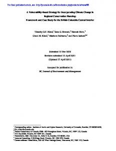
Figure 1. Pulsar searching workflow
Swinburne Astrophysics group has been conducting pulsar searching surveys using the observation data from Parkes Radio Telescope, which is one of the most famous radio telescopes in the world (http://www.parkes.atnf.csiro. au/). Pulsar searching is a typical scientific application. It contains complex and time consuming tasks and needs to process terabytes of data. Figure 1 depicts the high level structure of the pulsar searching workflow, which is currently running on Swinburne high performance supercomputing facility (http://astronomy.swin.edu.au/ supercomputing/). The description of detailed steps in this workflow can be found in our prior work [29]. At present, all the generated datasets are deleted after having been used, and the scientists only store the raw beam data, which are extracted from the raw telescope data. Whenever there are needs of using the deleted datasets, the scientists will regenerate them based on the raw beam files. The generated datasets are not stored, mainly because the
180
supercomputer is a shared facility that cannot offer unlimited storage capacity to hold the accumulated terabytes of data. However, some datasets are better to be stored. For example, the de-dispersion files, which are frequently used and the regeneration of these data will take more than 10 hours. It not only delays the scientists from conducting their experiments, but also requires a lot of computation resources. On the other hand, some datasets need not be stored. For example, the accelerated de-dispersion files, which are generated by the Accelerate step in Figure 1, are not often used. The Accelerate step is an optional step that is only for the binary pulsar searching. In light of this and given the large size of these datasets, they are not worth storing as it would be more cost effective to regenerate them from the de-dispersion files whenever used. Traditionally, scientific applications are deployed on high performance computing facilities, such as clusters and grids. How to store the generated datasets is normally decided by the scientists who launch the applications. This is because the clusters and grids normally only serve certain institutions. The scientists may store the datasets that are most valuable to them, based on the storage capacity of the system. However, in many scientific computing systems, the storage capacities are limited, such as the pulsar searching workflow example introduced earlier.
computation cost and storage cost may not be the best strategy for datasets storage. The storage strategy should be able to reflect these preferences from users about the computation delay in the cloud. Based on the discussion above, we need an effective datasets storage strategy for scientific applications in the cloud which can solve the following two problems: 1) reduce the total cost, and 2) take users’ preference into consideration. IV.
AN OVERVIEW OF SCIENTIFIC DATASETS STORAGE IN THE CLOUD
In this section, based on our prior work [27] [28] [29], we introduce some important concepts and enhance the representation of DDG and the datasets storage cost model in the cloud. A. Scientific application data in the cloud and DDG In general, there are two types of data stored in the cloud computing system, original data and generated data. 1) Original data are the data uploaded by users, and in scientific applications they are usually the raw data collected from the devices in the experiments. For these data, the users need to decide whether they should be stored or deleted, since they cannot be regenerated by the system once deleted. 2) Generated data are the data newly produced in the cloud computing system while the applications run. They are the intermediate or final computation results of the application which can be used in the future. For these data, their storage can be decided by the system, since they can be regenerated if their provenance is known. Hence, our datasets storage strategy is only applied to the generated data in the cloud computing environment that can automatically decide the storage status of generated datasets in scientific applications. In this paper, we refer generated data as dataset(s). DDG [29] is a directed acyclic graph (DAG) which is based on data provenance in scientific applications. All the datasets once generated in the system, whether stored or deleted, their references are recorded in the DDG. In other words, it depicts the generation relationships of datasets, with which the deleted datasets can be regenerated from its nearest existing preceding datasets. Figure 2 shows a simple DDG, where every node in the graph denotes a dataset. Dataset d1 pointing to d2 means that d1 is used to generate d2; and d2 pointing to d3 and d5 means d2 is used to generate d3 and d5 based on different operations; datasets d4 and d6 pointing to d7 means d4 and d6 are used together to generate d 7. We denote a dataset di in DDG as di ∈ DDG , and a set of datasets S={d1, d2 … dh} in DDG as S ⊆ DDG . To better describe the relationships of datasets in DDG, we define a symbol: → which denotes that two datasets have a generation relationship, where di → dj means di is a predecessor dataset of dj in the DDG. For example, in
B. Problem analysis In a commercial cloud computing environment [1], theoretically, the system can offer unlimited storage resources. All the datasets generated by the scientific applications can be stored, if the users are willing to pay for the required resources. Hence, for scientific applications in the cloud, whether to store the generated datasets or not is not an easy decision anymore. 1) Storing different datasets will lead to a very different cost. Due to the pay-as-you-go model, either storing or generating a dataset carries certain cost. The datasets vary in size, and have different generation costs and usage frequencies. On one hand, it is most likely not cost effective to store all these datasets in the cloud. On the other hand, if we delete them all, regeneration of frequently used datasets would normally impose a high computation cost. Hence we need a strategy to balance the generation cost and the storage cost of the application datasets in order to reduce the total application cost. Furthermore, single scientist cannot decide the datasets’ usages anymore, because for scientific applications in the cloud, datasets are shared among scientists from different institutions. Hence the datasets’ usages are determined by all the users and should be discovered and obtained from the system logs. 2) Data accessing delay should be considered for datasets storage in the cloud. Users have different preferences of storing the datasets, e.g. some users may want to store some datasets with higher storage cost to guarantee the immediate availability; some users may have tolerance of computation delay with a certain time. Hence, the best trade-off of
181
Figure 2’s DDG, we have d1 → d2, d1 → d4, d5 → d7, d1 → d7, etc. Furthermore, → is transitive, where di → d j → d k ⇔ di → d j ∧ d j → d k ⇒ di → d k .
cost per time unit of di in the system. The value CostRi depends on the storage status of di, where f i = stored y , CostRi = i genCost ( d ) ∗ v , f i = deleted i i
Hence, the total cost rate of storing a DDG, is the sum of CostR of all the datasets in it, which is ∑di ∈DDG CostRi . Given a time duration, the total cost of storing a DDG is the integral of the cost rate in this duration as a function of time t, which is Total _ Cost = ∫t (∑di ∈DDG CostRi ) • dt We further define the storage strategy of a DDG as S, where S ⊆ DDG , which means storing the datasets in S in the cloud and deleting the rest. We denote the cost rate of storing a DDG with the storage strategy S as
Figure 2. A simple Data Dependency Graph (DDG)
B. Datasets storage cost model in the cloud In a commercial cloud computing environment, if the users want to deploy and run applications, they need to pay for the resources used. The resources are offered by cloud service providers, who have their cost models to charge the users. In general, there are two basic types of resources in the cloud: storage and computation1. Popular cloud service providers’ cost models are based on these types of resources [1]. For example, Amazon cloud services’ prices are as follows: $0.15 per Gigabyte per month for the storage resources; $0.1 per CPU instance hour for the computation resources; In this paper, we define our datasets storage cost model in cloud computing system as follows: Cost = C + S , where the total cost of the system, Cost, is the sum of C, which is the total cost of computation resources used to regenerate datasets, and S, which is the total cost of storage resources used to store the datasets. To utilise the datasets storage cost model, we define the attributes for the datasets in the DDG same as in [29]. Briefly, for dataset di, its attributes are denoted as: , where • xi ($) denotes the generation cost of dataset di from its direct predecessors. • yi ($/t) denotes the cost of storing dataset di in the system per time unit. • fi (Boolean) is a flag, which denotes the status whether dataset di is stored or deleted in the system. • vi (Hz) denotes the usage frequency, which indicates how often di is used. • provSeti denotes the set of stored provenances that are needed when regenerating dataset di. Hence the generation cost of di is genCost (d i ) = xi + ∑{d k d j∈ provSeti ∧ d j →dk →di } xk
(∑ d ∈DDG CostRi )S i
Based on the definition above, different datasets storage strategies will lead to different cost rates to the system. Our strategy aims at reducing this cost rate. V.
LOCAL-OPTIMISATION BASED COST-EFFECTIVE DATASETS STORAGE STRATEGY
In this section, we improve the Cost Transitive Tournament Shortest Path (CTT-SP) algorithm that can find the minimum cost storage strategy for linear DDG with satisfying users’ tolerance of computation delay. Based on this algorithm, we further design a general localoptimisation based cost-effective storage strategy for scientific applications in the cloud. A. Improved CTT-SP algorithm for linear DDG CTT-SP algorithm was proposed in [29] which can find the minimum cost storage strategy of a given DDG with fixed datasets usages. The essence of CTT-SP algorithm is to construct a Cost Transitive Tournament (CTT) based on the DDG. In the CTT, the paths from the start dataset to the end dataset have a one-to-one mapping to the storage strategies of the DDG, and the length of the path equals to the total cost rate. Then we can use the well-known Dijkstra algorithm to find the shortest path, which is the minimum cost storage strategy. However, the CTT-SP algorithm for a general DDG is very complex, which carries the time complexity of O(n9). Hence we only adapt the CTT-SP algorithm for linear DDG to our strategy, which has the time complexity of O(n4). Linear DDG means a DDG with no branches, where all the datasets in the DDG only have one predecessor and one successor except the first and last datasets. In this section we will improve the linear CTT-SP algorithm that can reflect users’ tolerance of computation delay of accessing the datasets. We introduce another two attributes to represent users’ accessing delay tolerance of the datasets in the DDG. For dataset di, the attributes are denoted as: < Ti , λi >, where 1) Ti is a duration of time that denotes users’ tolerance of dataset di’s accessing delay.
• CostRi ($/t) is di’s cost rate, which means the average 1 Bandwidth is another common kind of resource in the cloud. In [13], Deelman et al. state that the cost-effective way of doing science in the cloud is to upload all the application data to the cloud storage and run all the applications with the cloud services. So we assume that the scientists upload all the original data to the cloud to conduct their experiments. Because transferring data within one cloud service provider’s facilities is usually free, the data transfer cost of managing the application datasets is not counted. In [29], the authors discussed the scenario of running scientific applications among different cloud service providers.
182
Users have tolerance of delay when they want to access a dataset. On one hand, one user may have different degrees of delay tolerance for different datasets. On the other hand, different users may also have different degrees of delay tolerance for one dataset. Ti is the minimum duration of delay that users can tolerant when accessing dataset di. In the linear CTT-SP algorithm, we have (∀d i , d j ∈ DDG ∧ d i → d j ) ⇒ ∃e < d i , d j > , and the weight of the edge, ω < d i , d j > means “the sum of cost rates of dj and the datasets between di and dj, supposing that only di and dj are stored and the rest of the datasets between di and dj are all deleted [29]”. However, in the improved linear CTT-SP algorithm, the edge e < d i , d j > has to further satisfy the condition
condition of users’ tolerance of regeneration time delay (lines 3 to 8). Next, we calculate the weight of the edges (lines 10 to 17), where we add the cost tolerance parameter λ (line 16). For the longest edge, the complexity of calculating its weight is O(n2) (lines 11 to 15), so a total of O(n4). Next, the Dijkstra algorithm has the time complexity of O(n2) (line 18). Hence, the improved linear CTT-SP algorithm also has a worst case time complexity of O(n4), and by adding the two new attributes, the algorithm can find the minimum cost storage strategy of DDG that satisfies users’ tolerance of datasets accessing delay.
genCost (d k ) ∀d k ∈ DDG ∧ (d i → d k → d j ) ∧ < Tk , CostCPU
where CostCPU is the price of CPU instances in the cloud. With this condition, many cost edges are eliminated from the CTT. It guarantees that in all storage strategies of the DDG found by the algorithm, for every deleted dataset di, its regeneration time is smaller than Ti. 2) λi is the parameter to denote users’ cost related tolerance of dataset di’s accessing delay, which is a value between 0 and 1. Sometimes, users prefer storing the datasets in the cloud to regenerating them even with a higher storage cost because of the accessing delay. To reflect this preference of users, in the improved linear CTT-SP algorithm the storage cost rate of the datasets will be multiplied by this parameter λ. The value of λ is set by the system manager based on users’ preference. The two extreme situations: λi=0 indicates no matter how large di ’s storage cost is, it has to be stored; λi=1 indicates the storage status of di only depends on its generation cost and storage cost in order to reduce the total system cost. Hence, in the improved linear CTT-SP algorithm, the weight of a cost edge in CTT is ω < d i , d j >= y j ∗ λ j + ∑{d k d k ∈DDG ∧di →d k →d j } ( genCost(d k ) ∗ v k ) In Figure 3, we demonstrate a simple example of constructing the CTT for a DDG that only has three datasets by the improved linear CTT-SP algorithm. Data dependency:
di → d j
di → d u → d j
e < di , d j >; di → d k → d j
di → d h → d k weight = weight + ( xk + genCost ) * vk ;
ω < d i , d j >= weight ;
Figure 4. Pseudo-code of CTT-SP algorithm
B. Local-optimisation based cost-effective datasets storage strategy In scientific applications, the relationships of the generated datasets are complex, i.e. one dataset could be used by different tasks and generate different datasets, and different datasets could also be used together to generate a new dataset, so that the DDG may have multiple branches. Given a general DDG with datasets’ usage frequencies derived from system logs, there also exists a minimum cost rate of storing it. We could further design more complex algorithms to find this minimum cost strategy, however we do not do this in our strategy mainly because of the dynamic nature of the cloud computing system explained as follows: 1) New datasets may be generated in the system at any time, so that the storage strategy needs to be triggered very frequently. This requires the algorithms in the strategy to be efficient. The algorithm of finding the minimum cost strategy of a general DDG is far more complex than the linear CTT-SP algorithm [29]; hence it is not suitable for the runtime datasets storage strategies. 2) The cost rate of storing a DDG calculated is a static value, which is based on the estimated datasets’ usage frequencies. The real cost rate for storing the datasets in
Cost edge: x1v1+(x1+x2)v2+(x1+x2+x3)v3
DDG d1
d2
d3
(x1 , y1 ,v1) (x2 , y2 ,v2) (x3 , y3 ,v3)
x1v1+(x1+x2)v2+y3*λ3
CTT ds
x3v3
x1v1+y2*λ2 y1*λ1
d1
y2*λ2
d2
y3*λ3
d3
0 de
x2v2+y3*λ3 x2v2+(x2+x3)v3
Figure 3. An example of constructing CTT
Based on the discussion above, we give the pseudo code of the improved linear CTT-SP algorithm in Figure 4. From the pseudo code in Figure 4, we can see that for a linear DDG with n datasets, we have to add a magnitude of n2 edges to construct the CTT (lines 1 to 2). In this improved linear CTT-SP algorithm, before actually creating the edge, we check whether this edge can satisfy the
183
cloud computing system is dynamic. Hence, it is unnecessary to design a very complex algorithm to find the minimum value for the runtime strategy. Next we will introduce our local-optimisation based datasets storage strategy, which is designed based on the improved linear CTT-SP algorithm. The philosophy is to derive localised minimum costs instead of a global one with low time complexity for the strategy. The strategy contains the following four rules: 1) Given a general DDG, the datasets to be stored first are the ones that users have no tolerance of accessing delay on them. This is to guarantee the immediate availability when these datasets are needed. 2) Then, the DDG is divided into separate sub DDGs by the stored datasets. For every sub DDG, if it is a linear one, we use the CTT-SP algorithm to find its storage strategy; otherwise, we find the datasets that have multiple direct predecessors or successors, and use these datasets as the partitioning points to divide it into sub linear DDGs, as shown in Figure 5 Then we use the improved linear CTT-SP algorithm to find their storage strategies. This is the essence of local optimisation.
in a general DDG is stored with its minimum cost storage strategy, hence achieves the local optimisation. VI.
EVALUATION
A. Simulation environment and strategies The datasets storage strategy proposed in this paper is generic. It can be used in any scientific applications with different price models of cloud services. In this section, we demonstrate the simulation results that we conduct on the SwinCloud environment [22]. First, we use general (random) DDG and datasets to demonstrate the costeffectiveness comparison of our strategy with others. Then we utilise our strategy to the specific pulsar searching application described in Section III, and use the real world data to demonstrate how our strategy works in storing the application datasets of the pulsar searching workflow. To evaluate the cost-effectiveness of our datasets storage strategy, we compare different storage strategies with our strategy. The representative strategies are: 1) Usage based strategy, in which we store the datasets that are most often used. 2) Generation cost based strategy, in which we store the datasets that incur the highest generation cost. 3) Cost rate based strategy reported in [27] [28], in which we store the datasets by comparing their own generation cost rate and storage cost rate. B. General random simulations and results The random simulations are conducted on randomly generated DDG with datasets of random sizes, generation times and usage frequencies. Due to the page limit, we only present some representative results in this section without losing generality. We use the DDG with 50 datasets, each with a random size from 100GB to 1TB. The generation time is also random, from 1 hour to 10 hours. The usage frequency is again randomly from 1 day to 10 days (time between every usage). The prices of cloud services follow the well-known Amazon’s cost model, i.e. $0.1 per CPU instance hour for computation2 and $0.15 per gigabyte per month for storage. To reflect users’ delay tolerance, we set a random time tolerance (Ti) from 10 hours to one day and a random cost parameter of delay tolerance (λi) from 0.7 to 1 to every datasets in the DDG. All these random parameters are generated with the uniform distribution. For other distributions, we have similar results in our experiment. To reflect the users’ preferences, we randomly select 4% of the datasets to store in the system based on users’ preferences. With the settings above, we ran simulations under different numbers of datasets in the DDG. Figure 6 shows the increases of the daily cost rates of different strategies as
Figure 5. Dividing a DDG into sub linear DDGs
3) When new datasets are generated in the system, they will be treated as a new sub DDG and added to the old DDG. Correspondingly, its storage status will be calculated in the same way as the old DDG. 4) When a dataset’s usage frequency is changed, we will re-calculate the storage status of the sub linear DDG that contains this dataset. In the strategy introduced above, the computation time complexity is well controlled within O(m*ni4) by dividing the general DDG into sub linear DDGs, where m is the number of the sub linear DDGs and ni is the number of datasets in the sub linear DDGs. In real applications, partition of a general DDG could be more flexible. The more segments we partition the DDG (i.e. ni becomes smaller), the more efficient but less cost-effective the strategy becomes. The extreme situation of ni =1 (i.e. every dataset is a segment) is the cost rate based strategy presented in [28] [27]. On the contrary, the other extreme situation of ni =N (i.e. the whole DDG) is the general CTT-SP algorithm presented in [29]. The suitable value of ni is application specific; hence we do not give detailed discussion in the paper due to the page limit. Hence our strategy has a feasible computation complexity in runtime of the system which depends on the size of the sub linear DDGs. The efficiency of running the strategy will be demonstrated in Section VI. Meanwhile, by utilising the CTT-SP algorithm, we guarantees that every sub linear DDG
2 Amazon cloud service offers different CPU instances with different prices, where using expensive CPU instances with higher performance would reduce computation time for some applications. There exists another important trade-off of time and cost [16] which is different with the tradeoff of computation and storage, hence is out of this paper’s scope.
184
the number of datasets grows in the DDG. From Figure 6, we can see that the “store none” and “store all” strategies are very cost ineffective, since their daily cost rates grow fast as the datasets number grows. The cost rate based strategy has a better performance than both the generation cost based strategy and usage based strategy. Our localoptimisation based strategy is the most cost-effective datasets storage strategy, and it reduces the total cost rate by over 20% on average comparing to the cost rate based strategy.
Section III and show how it works in this real world scientific application. In the pulsar example, for one execution of the workflow, six datasets are generated. Scientists may need to re-analyse these datasets, or reuse them in new workflows and generate new datasets. The DDG of this pulsar searching workflow is shown in Figure 8, as well as the sizes and generation times of these datasets. The generation times of the datasets are from running this workflow on Swinburne Astrophysics Supercomputer, and for simulation, we assume that in the cloud, the generation times of these datasets are the same. Furthermore, we again assume that the cost of cloud services follow Amazon clouds’ price.
Change of daily cost (4% users stored datasets) Store all datasets
Cost Rate (USD/Day)
2500
Store none
2000
1500
Usage based strategy
1000
Generation cost based strategy
500
Cost rate based strategy
0 0
100
200
300
400
500
600
700
800
900
1000 1100
Number of Datasets in DDG
Local-optimisation based strategy
Figure 6. Cost-effectiveness comparison of different storage strategies
Next we evaluate the efficiency and scalability of our local-optimisation based strategy by comparing the execution time with the cost rate based strategy and the original CTT-SP algorithm. We incorporate another two sets of simulations with different partition methods of the DDG, i.e. 1) we use the DDGs that only have 5 linear segments (m=5) and let the number of datasets in each segment grow; 2) we control the partition of the DDGs that every segment has at most 10 datasets (ni=10) and let the number of segments grow. In Figure 7, as the number of datasets increases, we can see that the original CTT-SP algorithm is not efficient; hence it can only be used for on-demand benchmarking. Although our strategy is not as simple as the cost rate based strategy, we deem that it is efficient and scalable for the datasets storage in runtime of the system. CPU Time of the strategies
Figure 8. DDG of the pulsar searching workflow
From Swinburne Astrophysics research group, we understand that the “De-dispersion files” is the most useful dataset. Based on these files, many accelerating and seeking methods can be used to search pulsar candidates. Based on the scenario, we set the “De-dispersion files” to be used once every 4 days and other datasets to be used once every 10 days. Furthermore, we assume new datasets are generated on the 10th day and 20th day, indicated as sub DDG1 and DDG2 in Figure 8. Based on this setting, we run the above mentioned simulation strategies and calculate the total costs of the system for one branch of the pulsar searching workflow of processing one piece of observation data in 30 days as shown in Figure 9. Figure 9 shows a consistent result with the previous general random simulations, where the cost rate based strategy also has a good performance in this pulsar searching application and the most cost-effective datasets storage strategy is still our local-optimisation based strategy.
Cost rate based strategy
200 180 160
Local-optimisation based strategy (n_i=10)
120 Local-optimisation based strategy
100
Total cost of 30 days - Pulsar case simulation
80 45
60 40 20 0 50
100
150
200
300
500
Local-optimisation based strategy (m=5)
40
CTT-SP algorithm
30
Store all datasets
Store none
35 Cost (USD)
Time(s)
140
1000
Number of datasets in DDG
Figure 7. Efficiency comparison of different storage strategies
Usage based strategy
25 20
Generation cost based strategy
15 10
C. Specific pulsar searching simulation and results The random simulations demonstrate the general performance of our datasets storage strategy. Next, we utilise it to the pulsar searching workflow introduced in
Cost rate based strategy
5 0 1
3
5
7
9 11 13 15 17 19 21 23 25 27 29 Days
Local-optimisation based strategy
Figure 9. Cost-effectiveness of our strategy in pulsar case DDG
185
VII.
CONCLUSIONS AND FUTURE WORK
In this paper, based on an astrophysics pulsar searching scientific application, we have examined the unique features of datasets storage in the cloud. We improved the CTT-SP (Cost Transitive Tournament Shortest Path) algorithm that can calculate the minimum cost rate of storing linear DDG in cloud computing systems, by taking into the consideration of users’ tolerance of data accessing delay. Based on the improved linear CTT-SP algorithm, we have developed a novel cost-effective datasets storage strategy that achieves a localised optimal trade-off of computation and storage cost of the cloud resources, with taking users’ preferences into consideration. Simulation results of utilising this strategy in both general (random) and specific pulsar searching application indicate that our strategy is efficient, scalable and cost-effective. In the future, more complex cost models and the model of estimating datasets usage frequencies need to be investigated, with which our strategy can be better adapted to different scientific applications in the cloud. Furthermore, the computation complexity of our strategy needs further investigation, where the cost of running the strategy itself should also be taken into consideration.
[13] [14]
[15] [16] [17] [18]
[19] [20]
[21]
ACKNOWLEDGMENT The research work reported here is partly supported by Australian Research Council under DP110101340. We are also grateful for the discussions on pulsar searching process with Dr. W. van Straten and Ms. L. Levin from Swinburne Centre for Astrophysics and Supercomputing.
[22]
[23]
REFERENCES [1] [2] [3] [4] [5] [6]
[7]
[8] [9] [10] [11]
[12]
"Amazon", http://aws.amazon.com/. "Eucalyptus", http://open.eucalyptus.com/. "Nimbus", http://www.nimbusproject.org/. "OpenNebula", http://www.opennebula.org/. I. Adams, D. D. E. Long, E. L. Miller, S. Pasupathy, and M. W. Storer, "Maximizing Efficiency by Trading Storage for Computation," in Workshop on Hot Topics in Cloud Computing, pp. 1-5, 2009. M. Armbrust, A. Fox, R. Griffith, A. D. Joseph, R. Katz, A. Konwinski, G. Lee, D. Patterson, A. Rabkin, I. Stoica, and M. Zaharia, "A View of Cloud Computing," Commun. ACM, vol. 53, pp. 50-58, 2010. M. D. d. Assuncao, A. d. Costanzo, and R. Buyya, "Evaluating the Cost-Benefit of Using Cloud Computing to Extend the Capacity of Clusters," in 18th ACM International Symposium on High Performance Distributed Computing, pp. 1-10, 2009. Z. Bao, S. Cohen-Boulakia, S. B. Davidson, A. Eyal, and S. Khanna, "Differencing Provenance in Scientific Workflows," in 25th IEEE International Conference on Data Engineering, pp. 808-819, 2009. R. Bose and J. Frew, "Lineage Retrieval for Scientific Data Processing: A Survey," ACM Comput. Surv., vol. 37, pp. 1-28, 2005. A. Burton and A. Treloar, "Publish My Data: A Composition of Services from ANDS and ARCS," in 5th IEEE International Conference on e-Science, pp. 164-170, 2009. R. Buyya, C. S. Yeo, S. Venugopal, J. Broberg, and I. Brandic, "Cloud Computing and Emerging IT Platforms: Vision, Hype, and Reality for Delivering Computing as the 5th Utility," Future Generation Computer Systems, vol. 25, pp. 599-616, 2009. E. Deelman, D. Gannon, M. Shields, and I. Taylor, "Workflows and e-Science: An Overview of Workflow System Features and
[24] [25]
[26] [27]
[28]
[29]
[30]
186
Capabilities," Future Generation Computer Systems, vol. 25, pp. 528540, 2009. E. Deelman, G. Singh, M. Livny, B. Berriman, and J. Good, "The Cost of Doing Science on the Cloud: the Montage Example," in ACM/IEEE Conference on Supercomputing, pp. 1-12, 2008. I. Foster, J. Vockler, M. Wilde, and Z. Yong, "Chimera: A Virtual Data System for Representing, Querying, and Automating Data Derivation," in 14th International Conference on Scientific and Statistical Database Management, pp. 37-46, 2002. I. Foster, Z. Yong, I. Raicu, and S. Lu, "Cloud Computing and Grid Computing 360-Degree Compared," in Grid Computing Environments Workshop, pp. 1-10, 2008. S. K. Garg, R. Buyya, and H. J. Siegel, "Time and Cost Trade-Off Management for Scheduling Parallel Applications on Utility Grids," Future Generation Computer Systems, vol. 26, pp. 1344-1355, 2010. P. Groth and L. Moreau, "Recording Process Documentation for Provenance," IEEE Transactions on Parallel and Distributed Systems, vol. 20, pp. 1246-1259, 2009. P. K. Gunda, L. Ravindranath, C. A. Thekkath, Y. Yu, and L. Zhuang, "Nectar: Automatic Management of Data and Computation in Datacenters," in 9th Symposium on Operating Systems Design and Implementation, pp. 1-14, 2010. G. Juve, E. Deelman, K. Vahi, and G. Mehta, "Data Sharing Options for Scientific Workflows on Amazon EC2," in ACM/IEEE Conference on Supercomputing, pp. 1-9, 2010. D. Kondo, B. Javadi, P. Malecot, F. Cappello, and D. P. Anderson, "Cost-Benefit Analysis of Cloud Computing versus Desktop Grids," in 23th IEEE International Parallel & Distributed Processing Symposium pp. 1-12, 2009. J. Li, M. Humphrey, D. Agarwal, K. Jackson, C. v. Ingen, and Y. Ryu, "eScience in the Cloud: A MODIS Satellite Data Reprojection and Reduction Pipeline in the Windows Azure Platform," in 24th IEEE International Parallel & Distributed Processing Symposium, pp. 1-12, 2010. X. Liu, D. Yuan, G. Zhang, J. Chen, and Y. Yang, "SwinDeW-C: A Peer-to-Peer Based Cloud Workflow System for Managing Instance Intensive Applications," in Handbook of Cloud Computing: Springer, pp. 309-332, 2010. B. Ludascher, I. Altintas, C. Berkley, D. Higgins, E. Jaeger, M. Jones, and E. A. Lee, "Scientific Workflow Management and the Kepler System," Concurrency and Computation: Practice and Experience, pp. 1039–1065, 2005. K.-K. Muniswamy-Reddy, P. Macko, and M. Seltzer, "Provenance for the Cloud," in 8th USENIX Conference on File and Storage Technology, pp. 197-210, 2010. L. J. Osterweil, L. A. Clarke, A. M. Ellison, R. Podorozhny, A. Wise, E. Boose, and J. Hadley, "Experience in Using A Process Language to Define Scientific Workflow and Generate Dataset Provenance," in ACM SIGSOFT International Symposium on Foundations of Software Engineering, pp. 319-329, 2008. A. S. Szalay and J. Gray, "Science in an Exponential World," Nature, vol. 440, pp. 23-24, 2006. D. Yuan, Y. Yang, X. Liu, and J. Chen, "A Cost-Effective Strategy for Intermediate Data Storage in Scientific Cloud Workflows," in 24th IEEE International Parallel & Distributed Processing Symposium, pp. 1-12, 2010. D. Yuan, Y. Yang, X. Liu, G. Zhang, and J. Chen, "A Data Dependency Based Strategy for Intermediate Data Storage in Scientific Cloud Workflow Systems," Concurrency and Computation: Practice and Experience, 2010. (http://dx.doi.org/10.1002/cpe.1636) D. Yuan, Y. Yun, X. Liu, and J. Chen, "On-demand Minimum Cost Benchmarking for Intermediate Datasets Storage in Scientific Cloud Workflow Systems," Journal of Parallel and Distributed Computing, vol. 72, pp. 316-332, 2011. M. Zaharia, A. Konwinski, A. D. Joseph, R. Katz, and I. Stoica, "Improving MapReduce Performance in Heterogeneous Environments," in 8th USENIX Symposium on Operating Systems Design and Implementation, pp. 29-42, 2008.